LogNormalDistribution
represents a lognormal distribution derived from a normal distribution with mean μ and standard deviation σ.
Details
- LogNormalDistribution is also known as the Galton distribution.
- LogNormalDistribution[0,1] is also known as Gibrat distribution.
- The lognormal distribution LogNormalDistribution[μ,σ] is equivalent to TransformedDistribution[Exp[x],xNormalDistribution[μ,σ]].
- LogNormalDistribution allows μ to be any real number and σ to be any positive real number.
- LogNormalDistribution allows μ and σ to be dimensionless quantities.
- LogNormalDistribution can be used with such functions as Mean, CDF, and RandomVariate. »
Background & Context
- LogNormalDistribution[μ,σ] represents a continuous statistical distribution supported over the interval
 and parametrized by a real number μ and by a positive real number σ that together determine the overall shape of its probability density function (PDF). Depending on the values of σ and μ, the PDF of a lognormal distribution may be either unimodal with a single "peak" (i.e. a global maximum) or monotone decreasing with a potential singularity approaching the lower boundary of its domain. In addition, the PDF of the lognormal distribution has tails that are "fat", in the sense that its PDF decreases algebraically rather than decreasing exponentially for large values of
  . (This behavior can be made quantitatively precise by analyzing the SurvivalFunction of the distribution.) The lognormal distribution is sometimes called the Galton distribution, the antilognormal distribution, or the Cobb–Douglas distribution.
 - LogNormalDistribution is the distribution followed by the logarithm of a normally distributed random variable. In other words, if
 is a random variable and
 ![XLogNormalDistribution[mu,sigma]](Files/LogNormalDistribution.en/4.png "XLogNormalDistribution[mu,sigma]") (where
(where  denotes "is distributed as"), then
 ![TemplateBox[{Log, paclet:ref/Log}, RefLink, BaseStyle -> {InlineFormula}][X]TemplateBox[{NormalDistribution, paclet:ref/NormalDistribution}, RefLink, BaseStyle -> {InlineFormula}][mu,sigma]](Files/LogNormalDistribution.en/6.png "TemplateBox[{Log, paclet:ref/Log}, RefLink, BaseStyle -> {InlineFormula}][X]TemplateBox[{NormalDistribution, paclet:ref/NormalDistribution}, RefLink, BaseStyle -> {InlineFormula}][mu,sigma]") . The origins of the lognormal distribution can be traced to an observation made by Francis Galton in the 1870s demonstrating that the distribution modeling the logarithm of a product of a number of independent positive random variates tends to a standard NormalDistribution as the number of variates gets infinitely large. The theory of the distribution was studied further in the early 1900s and has since been found to accurately model both the weights of humans and the sizes of computer files on a file system. In addition, the lognormal distribution has become a widely utilized tool for modeling various phenomena, including dust concentrations, gold and uranium grades, flood flows, lifetime distributions for manufactured products, and miscellaneous phenomena in finance and economics.
. The origins of the lognormal distribution can be traced to an observation made by Francis Galton in the 1870s demonstrating that the distribution modeling the logarithm of a product of a number of independent positive random variates tends to a standard NormalDistribution as the number of variates gets infinitely large. The theory of the distribution was studied further in the early 1900s and has since been found to accurately model both the weights of humans and the sizes of computer files on a file system. In addition, the lognormal distribution has become a widely utilized tool for modeling various phenomena, including dust concentrations, gold and uranium grades, flood flows, lifetime distributions for manufactured products, and miscellaneous phenomena in finance and economics. - RandomVariate can be used to give one or more machine- or arbitrary-precision (the latter via the WorkingPrecision option) pseudorandom variates from a lognormal distribution. Distributed[x,LogNormalDistribution[μ,σ]], written more concisely as xLogNormalDistribution[μ,σ], can be used to assert that a random variable x is distributed according to a lognormal distribution. Such an assertion can then be used in functions such as Probability, NProbability, Expectation, and NExpectation.
- The probability density and cumulative distribution functions for lognormal distributions may be given using PDF[LogNormalDistribution[μ,σ],x] and CDF[LogNormalDistribution[μ,σ],x]. The mean, median, variance, raw moments, and central moments may be computed using Mean, Median, Variance, Moment, and CentralMoment, respectively.
- DistributionFitTest can be used to test if a given dataset is consistent with a lognormal distribution, EstimatedDistribution to estimate a lognormal parametric distribution from given data, and FindDistributionParameters to fit data to a lognormal distribution. ProbabilityPlot can be used to generate a plot of the CDF of given data against the CDF of a symbolic lognormal distribution, and QuantilePlot to generate a plot of the quantiles of given data against the quantiles of a symbolic lognormal distribution.
- TransformedDistribution can be used to represent a transformed lognormal distribution, CensoredDistribution to represent the distribution of values censored between upper and lower values, and TruncatedDistribution to represent the distribution of values truncated between upper and lower values. CopulaDistribution can be used to build higher-dimensional distributions that contain a lognormal distribution, and ProductDistribution can be used to compute a joint distribution with independent component distributions involving lognormal distributions.
- LogNormalDistribution is related to a number of other distributions. It can be realized as a transformation of NormalDistribution, in the sense that the PDF of TransformedDistribution[Exp[x],xNormalDistribution[μ,σ]] is precisely the same as that of LogNormalDistribution[μ,σ]. Its logarithmic behavior is qualitatively similar to that of LogLogisticDistribution, LogMultinormalDistribution, and LogGammaDistribution. LogNormalDistribution is a special case of JohnsonDistribution. One can derive SuzukiDistribution by combining LogNormalDistribution with RayleighDistribution, in the sense that the PDF of SuzukiDistribution[μ,ν] is precisely the same as that of TransformedDistribution[u v,{uRayleighDistribution[1],vLogNormalDistribution[μ,ν]}]. By way of its connection to NormalDistribution, LogNormalDistribution is also related to StableDistribution, RiceDistribution, MaxwellDistribution, LevyDistribution, LaplaceDistribution, ChiDistribution, and ChiSquareDistribution.
Examples
open allclose allBasic Examples (4)
Scope (7)
Generate a sample of pseudorandom numbers from a log-normal distribution:
Compare the histogram to the PDF:
Distribution parameters estimation:
Estimate the distribution parameters from sample data:
Compare the density histogram of the sample with the PDF of the estimated distribution:
Skewness grows exponentially with standard deviation σ:
Kurtosis grows exponentially with standard deviation σ:
Different moments with closed forms as functions of parameters:
Applications (4)
Lognormal distribution can be used to model stock prices:
Fit the distribution to the data:
Compare the histogram to the PDF:
Find the probability that the price is above $500:
Simulate the price for the consecutive 30 days:
Lognormal distribution can be used to approximate wind speeds:
Find the estimated distribution:
Compare the PDF to the histogram of the wind data:
Find the probability of a day with wind speed greater than 30 km/h:
Simulate wind speeds for a month:
The fractional change of stock price ![]() at time
at time ![]() (in years) is assumed to be lognormally distributed with parameters
(in years) is assumed to be lognormally distributed with parameters ![]() and
and ![]() :
:
Compute expected stock price at epoch ![]() :
:
Assuming an investor can invest money for a year at a continuously compounded yearly rate ![]() risk-free, the risk-neutral pricing condition requires:
risk-free, the risk-neutral pricing condition requires:
Consider an option to buy this stock a year from now, at a fixed price ![]() . The value of such an option is:
. The value of such an option is:
The risk-neutral price of the option is determined as the present value of the expected option value:
Assuming rate ![]() of 5%, volatility parameter
of 5%, volatility parameter ![]() of 0.087, an initial price of $200 per share of stock, and a strike price of $190 per share, the Black–Scholes option price is:
of 0.087, an initial price of $200 per share of stock, and a strike price of $190 per share, the Black–Scholes option price is:
GammaDistribution data can be approximated by a lognormal distribution:
Comparing log-likelihoods with estimation by gamma distribution:
Properties & Relations (9)
Lognormal distribution is closed under scaling by a positive factor:
Power of a LogNormalDistribution follows a lognormal distribution:
In particular, a reciprocal of a lognormal distribution follows a lognormal distribution:
The product of two independent lognormally distributed variates follows lognormal distribution:
Quotient of two independent lognormally distributed variates follows lognormal distribution:
Geometric mean of independent identically lognormally distributed variates follows lognormal distribution:
Relationships to other distributions:
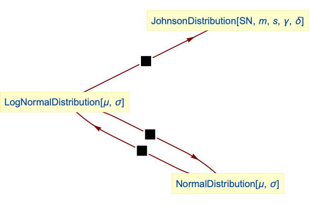
NormalDistribution is exponentially related to LogNormalDistribution:
Lognormal distribution is a special case of SL JohnsonDistribution:
SuzukiDistribution can be obtained from lognormal distribution and RayleighDistribution:
Possible Issues (2)
LogNormalDistribution is not defined when μ is not a real number:
LogNormalDistribution is not defined when σ is not a positive real number:
Substitution of invalid parameters into symbolic outputs gives results that are not meaningful:
Neat Examples (2)
LogNormalDistribution is not uniquely determined by its sequence of moments:
Compute the sequence of moments:
Compare it to the sequence of moments of the LogNormalDistribution:
Text
Wolfram Research (2007), LogNormalDistribution, Wolfram Language function, https://reference.wolfram.com/language/ref/LogNormalDistribution.html (updated 2016).
CMS
Wolfram Language. 2007. "LogNormalDistribution." Wolfram Language & System Documentation Center. Wolfram Research. Last Modified 2016. https://reference.wolfram.com/language/ref/LogNormalDistribution.html.
APA
Wolfram Language. (2007). LogNormalDistribution. Wolfram Language & System Documentation Center. Retrieved from https://reference.wolfram.com/language/ref/LogNormalDistribution.html