SliceContourPlot3D

SliceContourPlot3D[f,surf,{x,x_min,x_max},{y,y_min,y_max},{z,z_min,z_max}]

generates a contour plot of f over the slice surface surf as a function of x, y, and z.

SliceContourPlot3D[f,surf,{x,y,z}∈reg]

restricts the surface to be within region reg.

SliceContourPlot3D[f,{surf₁,surf₂,…},…]

generates contour plots over several slices.

Details and Options

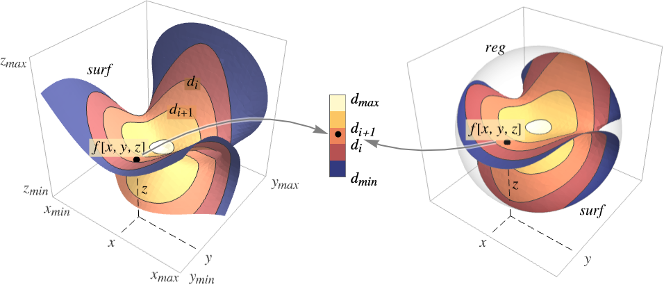
SliceContourPlot3D constructs contour curves on the surface surf corresponding to the level sets where f[x,y,z] has constant values d₁, d₂, etc. By default, the regions between the curves are shaded to more easily identify regions whose values are between d_i and d_i+1.
It visualizes the areas .

The following basic slice surfaces surf_i can be given:

		Automatic	automatically determine slice surfaces
		"CenterPlanes"	coordinate planes through the center
		"BackPlanes"	coordinate planes at the back of the plot
		"XStackedPlanes"	coordinate planes stacked along axis
		"YStackedPlanes"	coordinate planes stacked along axis
		"ZStackedPlanes"	coordinate planes stacked along axis
		"DiagonalStackedPlanes"	planes stacked diagonally
		"CenterSphere"	a sphere in the center
		"CenterCutSphere"	a sphere with a cutout wedge
		"CenterCutBox"	a box with a cutout octant

SliceContourPlot3D[f,{x,x_min,x_max},…] is equivalent to SliceContourPlot3D[f,Automatic,{x,x_min,x_max},…] etc.
The following parametrizations can be used for basic slice surfaces:

	{"XStackedPlanes",n},	generate n equally spaced planes
	{"XStackedPlanes",{x₁,x₂,…}}	generate planes for
	{"CenterCutSphere",ϕ_open}	cut angle ϕ_open facing the view point
	{"CenterCutSphere",ϕ_open,ϕ_center}	cut angle ϕ_open with center angle ϕ_center in the plane

"YStackedPlanes", "ZStackedPlanes" follow the specifications for "XStackedPlanes", with additional features shown in the scope examples.
The following general slice surfaces surf_i can be used:

	expr0	implicit equation in x, y, and z, e.g. x y z-10
	surfaceregion	a two-dimensional region in 3D, e.g. Hyperplane
	volumeregion	a three-dimensional region in 3D where surf_i is taken as the boundary surface, e.g. Cuboid

The following wrappers can be used for slice surfaces surf_i:

	Annotation[surf,label]	provide an annotation
	Button[surf,action]	define an action to execute when the surface is clicked
	EventHandler[surf,…]	define a general event handler for the surface
	Hyperlink[surf,uri]	make the surface act as a hyperlink
	PopupWindow[surf,cont]	attach a popup window to the surface
	StatusArea[surf,label]	display in status area when the surface is moused over
	Tooltip[surf,label]	attach an arbitrary tooltip to the surface

SliceContourPlot3D has the same options as Graphics3D, with the following additions and changes:

Axes	True	whether to draw axes
BoundaryStyle	Automatic	how to style surface boundaries
BoxRatios	{1,1,1}	bounding 3D box ratios
ClippingStyle	None	how to draw values clipped by PlotRange
ColorFunction	Automatic	how to color the plot
ColorFunctionScaling	True	whether to scale the arguments to ColorFunction
Contours	Automatic	how many or what contours to show
ContourShading	Automatic	how to shade regions between contours
ContourStyle	Automatic	the style for contour lines
PerformanceGoal	$PerformanceGoal	aspects of performance to optimize
PlotLegends	None	legends for color gradients
PlotPoints	Automatic	initial number of samples for the function f and slice surfaces surf_i in each direction
PlotRange	{Full,Full,Full,Automatic}	range of f or other values to include
PlotTheme	$PlotTheme	overall theme for the plot
RegionFunction	(True&)	how to determine whether a point should be included
ScalingFunctions	None	how to scale individual coordinates
TargetUnits	Automatic	desired units to use
WorkingPrecision	MachinePrecision	the precision used in internal computations

ColorFunction is by default supplied with the scaled value of f.
RegionFunction is by default supplied with x, y, z and f.
Possible settings for ScalingFunctions include:
s_f scale the f contour values

{s_x,s_y,s_z} scale x, y and z axes

{s_x,s_y,s_z,s_f} scale x, y and z axes and f contour values
Common built-in scaling functions s include:

	"Log"		log scale with automatic tick labeling
	"Log10"		base-10 log scale with powers of 10 for ticks
	"SignedLog"		log-like scale that includes 0 and negative numbers
	"Reverse"		reverse the coordinate direction
	"Infinite"		infinite scale

Examples

open allclose all

Basic Examples (2)

Plot the contours of the function over slice planes through the center:

Plot the contours over the surface :

Scope (24)

Surfaces (9)

Generate a contour plot over standard slice surfaces:

Standard axis-aligned stacked slice surfaces:

Standard boundary surfaces:

Plot the contours over any surface region:

Plotting over a volume primitive is equivalent to plotting over RegionBoundary[reg]:

Plot the contours over the surface :

Plot the contours over multiple surfaces:

Specify the number of stacked planes:

Specify the cutting angle for a center-cut sphere slice:

Sampling (4)

Use Contours to specify the number of contours:

Or the list of function values to put contours:

Areas where the function becomes nonreal are excluded:

Use RegionFunction to expose obscured slices:

The domain may be specified by a region including Cone:

A formula region including ImplicitRegion:

A mesh-based region including BoundaryMeshRegion:

Presentation (11)

Use PlotTheme to immediately get overall styling:

Use PlotLegends to get a color bar for the different values:

Control the display of axes with Axes:

Label axes using AxesLabel and the whole plot using PlotLabel:

Color the plot by the function values with ColorFunction:

Style regions between contours with ContourShading:

Use ContourStyle to style the contour lines:

Style the slice surface boundaries with BoundaryStyle:

TargetUnits specifies which units to use in the visualization:

Create a plot with a log-scaled axis:

Reverse the coordinate direction in the direction:

Options (43)

BoundaryStyle (1)

Style the slice surface boundaries with BoundaryStyle:

BoxRatios (3)

By default, the edges of the bounding box have the same length:

Use BoxRatios->Automatic to show the natural scale of the 3D coordinate values:

Use custom length ratios for each side of the bounding box:

ClippingStyle (2)

Color clipped regions:

Remove clipped regions with None:

ColorFunction (3)

Color the contours according to the values:

Use a named color gradient:

Use red when :

ColorFunctionScaling (2)

By default, scaled values are used:

Use ColorFunctionScalingFalse to get unscaled values:

Contours (4)

Use 5 equally spaced contours:

Use automatic contour selection:

Specify an explicit set of contours:

Use specific contours with specific styles:

ContourStyle (1)

Specify a style for all contours:

ContourShading (4)

ContourShadingAutomatic computes contour region shading from the ColorFunction:

Cyclically repeat shading styles:

Leave every third contour region empty, starting from the second:

Leave the regions between contours blank:

PerformanceGoal (2)

Generate a higher-quality plot:

Emphasize performance, possibly at the cost of quality:

PlotLegends (4)

Add a color bar for the different values:

PlotLegends automatically picks up Contours and ContourShading values:

With the setting ContourShadingAutomatic, the colors are derived from ColorFunction:

Control placement of the legend with Placed:

PlotPoints (1)

Use more plot points to get a smoother contour:

PlotRange (3)

Show All contours by default:

Show a select range:

Show only function values between 0 and 2:

This is equivalent to the fully qualified form:

PlotTheme (3)

Use a theme with detailed grid lines, ticks, and legends:

Any option setting overrides PlotTheme settings, in this case removing face grids:

Compare different plot themes:

RegionFunction (2)

Include only the contours where or :

Include only the contours where :

ScalingFunctions (5)

By default, plots have linear scales in all directions:

Create a plot with a log-scaled axis:

Use ScalingFunctions to scale to reverse the coordinate direction in the direction:

Use a scale defined by a function and its inverse:

Slice surfaces that are defined relative to the bounding box are unaffected by scaling functions:

TargetUnits (2)

Axes and legends are labeled with the units specified by TargetUnits:

Units specified by Quantity are converted to those specified by TargetUnits:

WorkingPrecision (1)

Evaluate functions using machine-precision arithmetic:

Applications (17)

Elementary Functions (4)

Plot the function :

Plot the functions and :

Plot , a product of univariate functions:

Plot and , univariate and bivariate functions:

Plot , a trivariate function:

Plot a sum of exponentials $sum_ialpha_i exp(-TemplateBox[{{p, -, {p, _, i}}}, Norm]^2)$ :

Pick the points randomly in a box:

Distribution Functions (6)

Plot the PDF of a distribution:

Simulate the distribution and show point distribution:

Plot the CDF of a distribution:

The SurvivalFunction:

The HazardFunction:

Explore Correlation parameters for a MultinormalDistribution, where ρ_ab is the correlation between a and b:

Correlation between x and y only:

Correlation between y and z only:

Correlation between y and z only, but larger variance in the z component:

Visualize the PDF of a ProductDistribution:

A product of three different distributions:

A product of bivariate and univariate distributions:

Plot the pdf of a CopulaDistribution:

Visualize the PDF of a kernel density estimate of some trivariate data:

Potential and Wave Functions (4)

Plot the phase using color on the isosurface of a quadrupole potential:

Alternatively, show the on several planes:

Plot spherical waves $cos(omega TemplateBox[{{p, -, {p, _, i}}}, Norm])$ from three sources in space:

Plot hydrogen orbital densities for quantum numbers , , :

Plot :

An electrostatic potential built from a collection of point charges at positions :

Two charges and :

Plot iso charge surfaces:

Show them together:

Partial Differential Equations (3)

Visualize a nonlinear sine-Gordon equation in two spatial dimensions with periodic boundary conditions with time represented along the z axis:

The solution evolves in time along the z axis:

Visualize Wolfram's nonlinear wave equation in two spatial dimensions with time represented along the z axis:

Visualize solutions to 3D partial differential equations. In this case, a Poisson equation over a Ball and Dirichlet boundary conditions:

Properties & Relations (5)

Use SliceDensityPlot3D for continuous densities on surfaces:

Use ContourPlot3D for constant value surfaces:

Use DensityPlot3D for full volume visualization of the function values:

Use ListSliceContourPlot3D for data:

Use ContourPlot for contour plots in 2D:

Possible Issues (1)

Slice surfaces with a constant value may appear noisy:

The function is constant on the chosen slice surface:

Choosing a different slice surface gives a reasonable picture of the function:

Top

SliceContourPlot3D

Details and Options

Examples

Basic Examples (2)