Search for all pages containing DSolve


DSolve
DSolve[eqn]
solves a differential equation eqn.
DSolve[eqn,u,x]
solves a differential equation for the function u, with independent variable x.
DSolve[eqn,u,{x,xmin,xmax}]
solves a differential equation for x between xmin and xmax.
DSolve[{eqn1,eqn2,…},{u1,u2,…},…]
solves a list of differential equations.
DSolve[eqn,u,{x1,x2,…}]
solves a partial differential equation.
DSolve[eqn,u,{x1,x2,…}∈Ω]
solves the partial differential equation eqn over the region Ω.
Details and Options
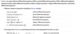
- DSolve can solve ordinary differential equations (ODEs), partial differential equations (PDEs), differential algebraic equations (DAEs), delay differential equations (DDEs), integral equations, integro-differential equations, and hybrid differential equations.
- Different classes of equations solvable by DSolve include:
-
u'[x]f[x,u[x]] ordinary differential equation a ∂xu[x,y]+b ∂yu[x,y]f partial differential equation f[u'[x],u[x],x]0 differential algebraic equation u'[x]f[x,u[x-x1]] delay differential equation u'[x]+  k[x,t]u[t]tf
integro-differential equation {…,WhenEvent[cond,u[x]g]} hybrid differential equation - The output from DSolve is controlled by the form of the dependent function u or u[x]:
-
DSolve[eqn,u,x] {{uf},…} where f is a pure function DSolve[eqn,u[x],x] {{u[x]f[x]},…} where f[x] is an expression in x - With a pure function output, eqn/.{{uf},…} can be used to verify the solution. »
- The dependent variable in DSolve[eqn] is inferred from eqn and may be specified either explicitly as u[x] or as a pure function u for autonomous equations. »
- DSolve can give implicit solutions in terms of Solve. »
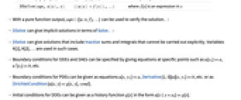
- DSolve can give solutions that include Inactive sums and integrals that cannot be carried out explicitly. Variables K[1], K[2], … are used in such cases.
- Boundary conditions for ODEs and DAEs can be specified by giving equations at specific points such as u[x1]a, u'[x2]b, etc.
- Boundary conditions for PDEs can be given as equations u[x,y1]a, Derivative[1,0][u][x,y1]b, etc. or as DirichletCondition[u[x,y]g[x,y],cond].
- Initial conditions for DDEs can be given as a history function g[x] in the form u[x/;x<x0]g[x].
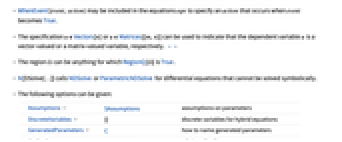
- WhenEvent[event,action] may be included in the equations eqn to specify an action that occurs when event becomes True.
- The specification u∈Vectors[n] or u∈Matrices[{m,n}] can be used to indicate that the dependent variable u is a vector-valued or a matrix-valued variable, respectively. Alternatively, u can be specified as a VectorSymbol or MatrixSymbol. » »
- The region Ω can be anything for which RegionQ[Ω] is True.
- N[DSolve[…]] calls NDSolve or ParametricNDSolve for differential equations that cannot be solved symbolically.
- The following options can be given:
-
Assumptions $Assumptions assumptions on parameters DiscreteVariables {} discrete variables for hybrid equations GeneratedParameters C how to name generated parameters Method Automatic what method to use IncludeSingularSolutions False whether to include singular solutions - GeneratedParameters controls the form of generated parameters; for ODEs and DAEs these are by default constants C[n] and for PDEs they are arbitrary functions C[n][…]. »
Examples
open all close allBasic Examples (3)
Solve a differential equation with dependent variable y[x]:
Get a "pure function" solution for y:
Substitute the solution into an expression:
Specify only the first argument of DSolve:
Solve the same equation with an implicit independent variable ![]() :
:
Scope (117)
Basic Uses (17)
Compute the general solution of a first-order differential equation:
Obtain a particular solution by adding an initial condition:
Plot the general solution of a differential equation:
Plot the solution curves for two different values of the arbitrary constant C[1]:
Solve a first-order differential equation using a one-argument specification:
Plot the solution of a boundary value problem:
Solve a boundary value problem using a one-argument specification:
Verify the solution of a first-order differential equation by using y in the second argument:
Obtain the general solution of a higher-order differential equation:
Solve a system of differential equations:
Solve a system of differential-algebraic equations:
Solve a system of differential equations using a one-argument specification:
Solve a partial differential equation:
Solve a partial differential equation using a one-argument specification:
Use different names for the arbitrary constants in the general solution:
Solve a delay differential equation:
Plot the solution for different values of the parameter:
Solve a hybrid differential equation:
This system models a bouncing ball:
Apply N[DSolve[...]] to invoke NDSolve if symbolic solution fails:
Linear Differential Equations (6)
Inhomogeneous first-order equation:
Solve a boundary value problem:
Second-order equation with constant coefficients:
Second-order equation with variable coefficients, solved in terms of elementary functions:
Equations with nonrational coefficients:
Solution in terms of hypergeometric functions:
Fourth-order equation solved in terms of Kelvin functions:
Linear equation with q-rational coefficients:
Higher-order inhomogeneous equation with constant coefficients:
Nonlinear Differential Equations (6)
Implicit solution for an Abel equation:
Solution in terms of WeierstrassP:
Systems of Differential Equations (8)
Inhomogeneous linear system with constant coefficients:
Linear system with rational function coefficients:
Solve a linear system of ODEs using vector variables:
Alternatively, define ![]() as a VectorSymbol:
as a VectorSymbol:
Solve a linear system of four ODEs using matrix variables:
Alternatively, define ![]() as a MatrixSymbol:
as a MatrixSymbol:
Solve inhomogeneous linear system of ODEs with constant coefficients:
Differential-Algebraic Equations (3)
Delay Differential Equations (2)
Piecewise Differential Equations (4)
Using a piecewise forcing function:
A differential equation with a piecewise coefficient:
A nonlinear piecewise-defined differential equation:
Differential equations involving generalized functions:
A simple impulse response or Green's function:
Solve a piecewise differential equation on the interval {0,1}:
Hybrid Differential Equations (8)
Solve a first-order differential equation with a time-dependent event:
Solve a second-order differential equation with a time-dependent event:
Solve a system of differential equations with a state-dependent event:
Stop the integration when an event occurs:
Remove an event after it has occurred once:
Specify that a variable maintains its value between events:
Sturm-Liouville Problems (6)
Solve an eigenvalue problem with Dirichlet conditions:
Make a table of the first 5 eigenfunctions:
Solve an eigenvalue problem with Neumann conditions:
Make a table of the first 5 eigenfunctions:
Solve an eigenvalue problem with mixed boundary conditions:
Make a table of the first 5 eigenfunctions:
Solve an eigenvalue problem with a Robin condition at the left end of the interval:
Locate the roots of the transcendental eigenvalue equation in the range 10<λ<80:
Obtain the eigenfunctions within this range by using Assumptions:
Solve an eigenvalue problem with Robin boundary conditions at both ends:
Solve an eigenvalue problem for the Airy operator:
Integral Equations (6)
Solve a Volterra integral equation:
Solve a Fredholm integral equation:
Solve an integro-differential equation:
Specify an initial condition to obtain a particular solution:
Solve a singular Abel integral equation:
Solve a weakly singular Volterra integral equation:
First-Order Partial Differential Equations (7)
General solution for a linear first-order partial differential equation:
The solution with a particular choice of the arbitrary function C[1]:
Initial value problem for a linear first-order partial differential equation:
Initial-boundary value problem for a linear first-order partial differential equation:
General solution for the transport equation:
Plot the traveling wave with speed c1:
General solution for a quasilinear first-order partial differential equation:
Initial value problem for a scalar conservation law:
Complete integral for a nonlinear first-order Clairaut equation:
Hyperbolic Partial Differential Equations (11)
Initial value problem for the wave equation:
The wave propagates along a pair of characteristic directions:
Initial value problem for the wave equation with piecewise initial data:
Discontinuities in the initial data are propagated along the characteristic directions:
Initial value problem with a pair of decaying exponential functions as initial data:
Initial value problem for an inhomogeneous wave equation:
Visualize the solution for different values of m:
Initial value problem for the wave equation with a Dirichlet condition on the half-line:
The wave bifurcates starting from the initial data:
Initial value problem for the wave equation with a Neumann condition on the half-line:
In this example, the wave evolves to a non-oscillating function:
Dirichlet problem for the wave equation on a finite interval:
The solution is an infinite trigonometric series:
Extract the first three terms from the Inactive sum:
The wave executes periodic motion in the vertical direction:
Dirichlet problem for the wave equation in a rectangle:
The solution is a doubly infinite trigonometric series:
Extract a few terms from the Inactive sum:
The two-dimensional wave executes periodic motion in the vertical direction:
Dirichlet problem for the wave equation in a circular disk:
The solution is an infinite Bessel series:
Extract the first three terms from the Inactive sum:
General solution for a second-order hyperbolic partial differential equation:
Hyperbolic partial differential equation with non-rational coefficients:
Inhomogeneous hyperbolic partial differential equation with constant coefficients:
Initial value problem for an inhomogeneous linear hyperbolic system with constant coefficients:
Parabolic Partial Differential Equations (7)
Initial value problem for the heat equation:
Visualize the diffusion of heat with the passage of time:
Initial value problem for the heat equation with piecewise initial data:
The solution is given in terms of the error function Erf:
Discontinuities in the initial data are smoothed instantly:
Initial value problem for an inhomogeneous heat equation:
Visualize the growth of the solution for different values of the parameter m:
Dirichlet problem for the heat equation on a finite interval:
The solution is a Fourier sine series:
Extract three terms from the Inactive sum:
Neumann problem for the heat equation on a finite interval:
The solution is a Fourier cosine series:
Extract a few terms from the Inactive sum:
Visualize the evolution of the solution to its steady state:
Dirichlet problem for the heat equation in a disk:
The solution is an infinite Bessel series:
Extract a few terms from the Inactive sum:
Visualize the individual terms of the solution at time t=0.1:
Elliptic Partial Differential Equations (9)
Dirichlet problem for the Laplace equation in the upper half-plane:
Discontinuities in the boundary data are smoothed out:
Dirichlet problem for the Laplace equation in the right half-plane:
Dirichlet problem for the Laplace equation in the first quadrant:
Neumann problem for the Laplace equation in the upper half-plane:
Dirichlet problem for the Laplace equation in a rectangle:
The solution is an infinite trigonometric series:
Extract a few terms from the Inactive sum:
Dirichlet problem for the Laplace equation in a disk:
Dirichlet problem for the Laplace equation in an annulus:
Dirichlet problem for the Poisson equation in a rectangle:
Dirichlet problem for the Helmholtz equation in a rectangle:
Extract a finite number of terms from the Inactive sum:
General Partial Differential Equations (6)
A potential-free Schrödinger equation with Dirichlet boundary conditions:
Extract the first four terms in the solution:
For any choice of the four constants C[k], ψ obeys the equation and boundary conditions:
Initial value problem for a Schrödinger equation with Dirichlet boundary conditions:
Define a family of partial sums of the solution:
For each k, uk satisfies the differential equation:
The boundary conditions are also satisfied:
The initial condition is only satisfied for u∞, but there is rapid convergence at t==2:
Solve a Schrödinger equation with potential over the reals:
Extract the first two terms in the solution:
For any values of the constants C[0] and C[1], the equation is satisfied:
The conditions at infinity are also satisfied:
Although the function is time dependent, its ![]() -norm is constant:
-norm is constant:
Initial value problem for Burgers' equation with viscosity ν:
Plot the solution at different times for ν=1/40:
Plot the solution for different values of ν:
Boundary value problem for the Tricomi equation:
Traveling wave solution for the Korteweg–de Vries (KdV) equation:
Obtain a particular solution for a fixed choice of arbitrary constants:
Partial Differential Equations over Regions (3)
Dirichlet problem for the Laplace equation in a rectangle:
Extract the first 100 terms from the Inactive sum:
Visualize the solution on the rectangle:
Dirichlet problem for the Laplace equation in a disk:
Visualize the solution in the disk:
Dirichlet problem for the Laplace equation in a right half-plane:
Fractional Differential Equations (8)
Solve a fractional differential equation of order 1/2:
Solve a fractional differential equation containing CaputoD of order 0.7:
Add initial conditions and plot the solution:
Solve a fractional differential equation containing two Caputo derivatives of different orders:
Solve a non-homogeneous fractional differential equation of order 1/7:
Solve a system of two fractional differential equations:
Parametrically plot the solution:
Solve a system of two fractional ODEs in vector form:
Parametrically plot the solution:
Solve a system of three fractional differential equations in vector form:
Generalizations & Extensions (1)
Options (7)
Assumptions (2)
Solve an eigenvalue problem for a linear second-order differential equation:
Use Assumptions to specify a range for the parameter λ:
Specify that the independent variable x is real:
Obtain the same result using an interval specification for x:
GeneratedParameters (2)
Use differently named constants:
Generate uniquely named constants of integration:
The constants of integration are unique across different invocations of DSolve:
Method (1)
Solve a linear ordinary differential equation:
Obtain a solution in terms of DifferentialRoot:
SingularSolutions (1)
By default, DSolve returns the general solution for this ODE:
Use IncludeSingularSolutions to compute singular solutions along with the general solution:
Applications (36)
Ordinary Differential Equations (12)
Solve a logistic (Riccati) equation:
Plot the solution for different initial values:
Solve a linear pendulum equation:
Displacement of a linear, damped pendulum:
Study the phase portrait of a dynamical system:
Find a power series solution when the exact solution is known:
Verify that y=0 and y=1 are equilibrium solutions of the logistic equation:
Model a block on a moving conveyor belt anchored to a wall by a spring. Compare positions and velocities for the different values of the parameters of the system (mass of the block, belt speed, friction coefficient, spring constant):
Newton's equation for the block:
Solve for position and velocity:
The block stabilizes just above the spring's natural length of l:
Use component laws together with Kirchhoff's laws for connections to simulate the response of an RLC circuit to a step impulse in the voltage ![]() applied at time
applied at time ![]() :
:
The component laws read ![]() ,
, ![]()
![]() ,
, ![]() and
and ![]() :
:
Visualize the response for different values of ![]() ,
, ![]() and
and ![]() :
:
Model the change in height of water in two cylindrical tanks as water flows from one tank to another through a pipe:
Use pressure relations ![]() and mass conservation:
and mass conservation:
Model the flow across the pipe with the Hagen–Poiseuille relation:
Visualize the solution for particular values of the parameters:
Solve the equation of a fractional harmonic oscillator of order 1.9:
A fractional harmonic oscillator behaves like a damped harmonic oscillator:
Fit the data for a fractional oscillator with the solution of a damped oscillator to determine the corresponding value for damping factor ![]() :
:
Solve the equation of fractional LC electric circuit:
The classical solution can be obtained for ![]() :
:
Solve the LC circuit equation for ![]() :
:
Plot the solutions for various values of equation order ![]() :
:
Solve the equation of fractional RC electric circuit:
The classical solution can be obtained for ![]() :
:
Hybrid Differential Equations (8)
Model a damped oscillator that gets a kick at regular time intervals:
Model a ball bouncing down steps:
In a square box, model a ball that changes direction upon impact with the side walls:
Simulate the system ![]() stabilized with a discrete-time controller
stabilized with a discrete-time controller ![]() :
:
Control a double integrator using a dead-beat, discrete-time controller:
Use a dead-beat digital feedback controller ![]() :
:
Model the position of a moving body with 1 kg mass:
Use a sampled proportional-derivative (PD) controller to keep the position constant:
Set the physical variable a to 0 whenever it becomes negative:
Delay Differential Equations (2)
Integral Equations (4)
The tautochrone problem requires finding the curve down which a bead placed anywhere will fall to the bottom in the same amount of time. Expressing the total fall time in terms of the arc length of the curve and the speed v yields the Abel integral equation ![]() . Defining the unknown function
. Defining the unknown function ![]() by the relationship
by the relationship ![]() and using the conservation of energy equation
and using the conservation of energy equation ![]() yields the explicit equation:
yields the explicit equation:
Use DSolve to solve the integral equation:
Using the relationship ![]() , solve for
, solve for ![]() :
:
Starting the curve from the origin and integrating—with assumptions that ensure the integrand is real-valued—yields ![]() as a function of
as a function of ![]() :
:
Substituting values for ![]() and
and ![]() , use ParametricPlot to display the maximal tautochrone curve:
, use ParametricPlot to display the maximal tautochrone curve:
Making the change of variables ![]() gives a simple, nonsingular parametrization of the curve with
gives a simple, nonsingular parametrization of the curve with ![]() :
:
Combining the conservation of energy equation and the chain rule ![]() produces the following differential equation for
produces the following differential equation for ![]() as a function of
as a function of ![]() :
:
This equation can be solved numerically for different starting points:
Plotting the solutions shows that all reach the bottom, ![]() , at the two-second mark:
, at the two-second mark:
Visualize the motion along the tautochrone:
A spring-mass system, with an attached mass of
, has a spring constant of and a damping coefficient of . At timeInitial value of the velocity:
Solve the integro-differential equation using DSolve:
Plot the velocity as a function of time:
Visualize the motion of the physical spring-mass system:
An LRC circuit has a voltage source given by ![]() . The resistance in the circuit is 0.2
. The resistance in the circuit is 0.2 ![]() , the inductance is
, the inductance is
The integral equation for the current is given by:
Solve the integro-differential equation using DSolve:
Plot the current as a function of time:
A linear Volterra integral equation is equivalent to an initial value problem for a linear differential equation. Verify this relationship for the following Volterra equation:
Solve the integral equation using DSolve:
Set up the corresponding differential equation:
Add two initial conditions since the differential equation is of second order:
The solution of the initial value problem agrees with that of the integral equation:
Classical Partial Differential Equations (5)
Model the vibrations of a string with fixed length, say π, using the wave equation:
Specify that the ends of the string remain fixed during the vibrations:
Obtain the fundamental and higher harmonic modes of oscillation:
Visualize the vibrations of the string for these modes:
In general, the solution is composed of an infinite number of harmonics:
Extract four terms from the Inactive sum:
Visualize the vibration of the string:
Model the oscillations of a circular membrane of radius 1 using the wave equation in 2D:
Specify that the boundary of the membrane remain fixed:
Initial condition for the problem:
Obtain a solution in terms of Bessel functions:
Extract a finite number of terms from the Inactive sum:
Visualize the oscillations of the membrane:
Model the flow of heat in a bar of length 1 using the heat equation:
Specify the fixed temperature at both ends of the bar:
Solve the heat equation subject to these conditions:
Extract a few terms from the Inactive sum:
Visualize the evolution of the temperature to a steady state:
Obtain the steady-state solution v[x], which is independent of time:
The steady-state solution is a linear function of x:
Model the flow of heat in a bar of length 1 that is insulated at both ends:
Specify that no heat flow through the ends of the bar:
Solve the heat equation subject to these conditions:
Extract a few terms from the Inactive sum:
Visualize the evolution of the temperature to the steady-state value of 60°:
Construct a complex analytic function, starting from the values of its real and imaginary parts on the ![]() axis. The real and imaginary parts u and v satisfy the Cauchy–Riemann equations:
axis. The real and imaginary parts u and v satisfy the Cauchy–Riemann equations:
Prescribe the values of u and v on the ![]() axis:
axis:
Solve the Cauchy–Riemann equations:
Verify that the solutions are harmonic functions:
Visualize the streamlines and equipotentials generated by the solution:
General Partial Differential Equations (5)
Study the evolution of a smooth solution for Burgers' equation to a shock wave in the limit when the viscosity parameter becomes infinitely small:
The solution is smooth for any positive value of ϵ:
The solution develops a shock discontinuity in the limit when ϵ approaches 0:
An electron constrained to move in a one-dimensional box of length d is governed by the free Schrödinger equation with Dirichlet conditions at the endpoints:
The general solution to this equation is a sum of trigonometric-exponential terms:
Each term in the sum is called a stationary state, as using the sine as initial conditions leads to the positional probability density ![]() being time independent. For example:
being time independent. For example:
The resulting probability distribution is independent of time:
The normalization of the initial data was chosen so that the integral of the density (the total probability of finding the particle somewhere) is 1:
Using any other initial condition, even one as simple as a sum of two stationary states, will lead to a complicated, time-dependent density:
This density is not stationary, as t appears in the second and third cosines:
Although the probability density is time dependent, its integral is still the constant 1:
Entering the mass of the electron and the value of ![]() in SI units and setting d to a typical interatomic distance of 1 nm results in the following density function:
in SI units and setting d to a typical interatomic distance of 1 nm results in the following density function:
Visualize the function over the spatial domain and one period in time:
Viewing the graph as a movie of probability densities, it can be seen that "center" of the electron moves from side to side of the box:
Find the value of a European vanilla call option if the underlying asset price and the strike price are both $100, the risk-free rate is 5%, the volatility of the underlying asset is 20%, and the maturity period is 1 year, using the Black–Scholes model:
Solve the boundary value problem:
Compute the value of the European vanilla option:
Compare with the value given by FinancialDerivative:
Recover a function from its gradient vector:
The solution represents a family of parallel surfaces:
Properties & Relations (10)
Solutions satisfy the differential equation and boundary conditions:
Differential equation corresponding to Integrate:
Use NDSolve to find a numerical solution:
Use DEigensystem to find eigenvalues and eigenfunctions:
Find the complete eigensystem:
Find eigenvalues and eigenfunctions:
Compute an impulse response using DSolve:
The same computation using InverseLaplaceTransform:
DSolve returns a rule for the solution:
DSolveValue returns an expression for the solution:
Apply N[DSolve[...]] to invoke NDSolve if symbolic solution fails:
Solve the Laplace equation in a rectangle:
Obtain the same result using the region notation:
Use DFixedPoints to find the fixed points of a system of two ODEs:
Use DStabilityConditions to analyze the stability of the fixed point:
Solve the system using the fixed point as initial condition:
Solve the system for given initial conditions:
Use system modeling for numerical solutions to larger hierarchical models:
Possible Issues (9)
Results may contain inactive integrals:
Replacing the function ![]() by an expression still returns inactive integrals:
by an expression still returns inactive integrals:
Use Activate to evaluate integrals:
Capital ![]() and capital
and capital ![]() cannot be used as independent variables:
cannot be used as independent variables:
Replacing them by lowercase ![]() or lowercase
or lowercase ![]() fixes the issue:
fixes the issue:
Inverse functions may be required to find the solution:
Definitions for an unknown function may affect the evaluation:
Clearing the definition for the unknown function fixes the issue:
Here DSolve gives an error message because ![]() is not included in the second argument:
is not included in the second argument:
Include ![]() in the second argument to obtain a solution:
in the second argument to obtain a solution:
Alternatively, use DSolveValue to obtain the solution for ![]() alone:
alone:
This example returns unevaluated because DSolve is unable to interpret it as a vector equation:
The example can be solved by rewriting it as follows:
CompleteIntegral finds a complete integral for a nonlinear PDE:
DSolve returns the same solution with a warning message:
Use CompleteIntegral to find a complete integral for a linear PDE:
DSolve returns the general solution for this PDE:
Solve a second-order linear ODE with symbolic parameters:
The solution obtained is not the general solution of the ODE for specific values of parameters ![]() :
:
The general solution for this case can be found by substituting parameter values in the equation first:
Text
Wolfram Research (1991), DSolve, Wolfram Language function, https://reference.wolfram.com/language/ref/DSolve.html (updated 2025).
CMS
Wolfram Language. 1991. "DSolve." Wolfram Language & System Documentation Center. Wolfram Research. Last Modified 2025. https://reference.wolfram.com/language/ref/DSolve.html.
APA
Wolfram Language. (1991). DSolve. Wolfram Language & System Documentation Center. Retrieved from https://reference.wolfram.com/language/ref/DSolve.html