Helmholtz Resonator
| Introduction | Acoustic Model |
| Domain | Wine Bottle as a Helmholtz Resonator |
| Model Setup | Nomenclature |
| Boundary Conditions | References |
Introduction
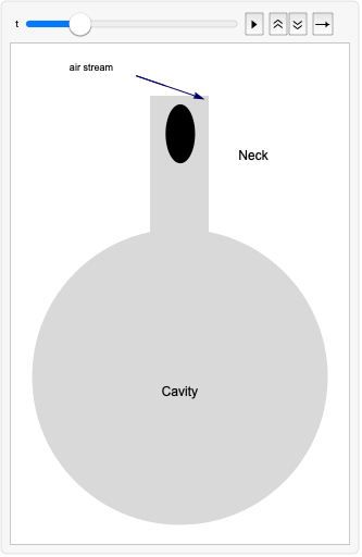
When one blows carefully across the opening of a bottle, a clear sound is generated. The sound is generated by oscillations in the air stream passing over the far edge of the opening.
The bottle is composed of an opening called the mouth, a narrow volume called the neck and a large volume called the cavity. Conceptually speaking, by blowing over the mouth of the bottle, the inert mass of the air in the neck is pushed inward into the cavity. This compresses the air in the cavity and increases the pressure in the cavity. At a certain point, the pressure in the cavity is high enough to push the inert mass of air in the neck back up and beyond its initial position outside. This then directs the flow of air across the mouth to flow over the edge. The air stream over the bottle then pushes the air in the neck back down and the cycle repeats. The air stream alternates quickly between going inside the bottle and going over the bottle and produces the sound.
The oscillation of the air stream happens at a specific frequency defined by the geometry of the bottle. This frequency is called the Helmholtz resonance frequency. To model this phenomenon, the theory describing a Helmholtz resonator can be used. While the geometry of a Helmholtz resonator is different from a bottle, the same theoretical concepts can be applied.
Helmholtz resonators are commonly used to suppress noise in ducts of ventilation systems and exhaust pipes of combustion engines [Li, et al., 2017].
A different way to understand the functioning of the Helmholtz resonator is by an analogy to a mechanical mass-spring system or electrical inductance-capacitance system. The mass (inductance) and spring (capacitance) are in series. In this conceptual model, the air in the neck acts as a mass (inductance), and air in the cavity is like a spring (capacitance) [Rahim & Johari, 2016].
Since the value of resistance does not affect the resonance frequency, in this notebook an axisymmetric Helmholtz resonator is simulated without resistance, with the goal of reproducing the resonator frequency response.
Domain
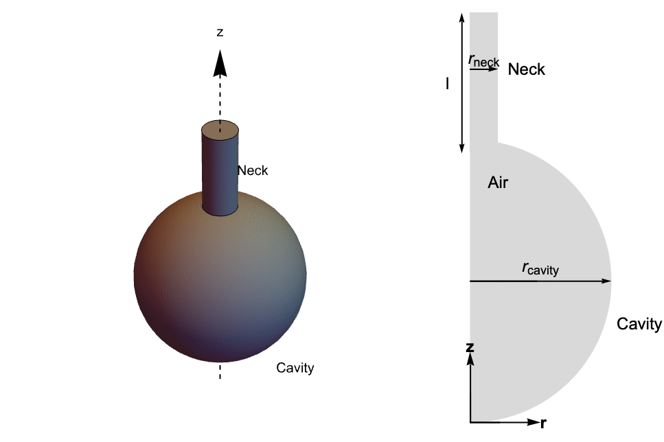
The bottle geometry consists of a neck of length ![]() and radius
and radius ![]() and a spherical cavity of radius
and a spherical cavity of radius ![]() . Since this oscillator is rotationally symmetric about the
. Since this oscillator is rotationally symmetric about the ![]() axis, the geometry can be approximated by its 2D cross section in the
axis, the geometry can be approximated by its 2D cross section in the ![]() plane. The figures below illustrate the simulation domain.
plane. The figures below illustrate the simulation domain.
Model Setup
The system will be modeled in the frequency domain to analyze its frequency response. The main PDE model of acoustics in the frequency domain is the Helmholtz equation. Since the domain and the boundary conditions are rotationally symmetric about the ![]() axis, an axisymmetric PDE model can be used. The axisymmetric Helmholtz equation is used to solve for the pressure field
axis, an axisymmetric PDE model can be used. The axisymmetric Helmholtz equation is used to solve for the pressure field ![]() in
in ![]() and to describe the propagation of harmonic sound waves at different frequencies.
and to describe the propagation of harmonic sound waves at different frequencies.
The axisymmetric Helmholtz equation is given as:
where ![]() is the density in
is the density in ![]() ,
, ![]() is the speed of sound in the medium
is the speed of sound in the medium ![]() , and
, and ![]() is the angular frequency
is the angular frequency ![]() .
.
The axisymmetric Helmholtz equation uses a truncated cylindrical coordinate system in 2D with independent variables ![]() instead of the cylindrical coordinates
instead of the cylindrical coordinates ![]() . The cylindrical coordinate variable
. The cylindrical coordinate variable ![]() disappears because the system is rotationally symmetric about the
disappears because the system is rotationally symmetric about the ![]() axis.
axis.
The AcousticPDEComponent function can produce the axisymmetric form of the Helmholtz equation. To do so, the parameter "RegionSymmetry" is set to "Axisymmetric".
The goal is to obtain the frequency response of the oscillator. For this, the system is analyzed over a range of frequencies, and the pressure levels at those frequencies are recorded. The frequency sweep will be with ![]() frequencies ranging from
frequencies ranging from ![]() to
to ![]() that are evenly spaced using a log scale. This range of frequencies allows one to see the different harmonics of the system.
that are evenly spaced using a log scale. This range of frequencies allows one to see the different harmonics of the system.
The next section shows how to compute and visualize the frequency response of the system.
Resonance Frequency
As mentioned before, the Helmholtz resonator can be viewed as equivalent to an oscillatory system. In electrical terminology, the system behaves like an ![]() circuit in series. So, taking the
circuit in series. So, taking the ![]() circuit analogy, one can find that the resonance frequency is given by [Blackstock, 2001]:
circuit analogy, one can find that the resonance frequency is given by [Blackstock, 2001]:
where the parameters ![]() and
and ![]() are given by:
are given by:
Here, ![]() is the density of the medium,
is the density of the medium, ![]() is the speed of sound in the medium,
is the speed of sound in the medium, ![]() is the cross-sectional area of the neck,
is the cross-sectional area of the neck, ![]() is the volume of the acoustic cavity and
is the volume of the acoustic cavity and ![]() is the total length of the neck.
is the total length of the neck.
As mentioned before, there exists a restoring force that causes the mass of air to leave the neck. This small distance covered by the mass of air is considered in the theory to still be part of the tube, as if the air had always remained inside the neck. This distance is added to the original neck length as a correction factor ![]() . Therefore, if the original length of the neck is
. Therefore, if the original length of the neck is ![]() , then the total length
, then the total length ![]() equals
equals ![]() .
.
The correction length of the neck depends on the geometry of the connection between the neck and the cavity. Here, the correction length will be assumed to be ![]() [Pierce, 2019].
[Pierce, 2019].
With the above definitions, one finds that the Helmholtz resonance frequency is given by:
where in the last equation, the assumption is made that the volume is from a sphere with ![]() and the neck cross-sectional area is
and the neck cross-sectional area is ![]() .
.
The resonance frequency ![]() is part of the frequency range, fRange, for the frequency sweep.
is part of the frequency range, fRange, for the frequency sweep.
Boundary Conditions
At the mouth of the oscillator, a harmonically oscillating pressure ![]() is applied with
is applied with ![]() . At the rest of the boundaries, a sound hard boundary condition is applied, and as this is the natural default boundary condition, this can be left out.
. At the rest of the boundaries, a sound hard boundary condition is applied, and as this is the natural default boundary condition, this can be left out.
Acoustic Model
In acoustics simulations, the wavelength ![]() of a sound wave needs to be resolved by a sufficiently fine mesh in order to get an accurate numerical solution. Here a helper function is used to set the MaxCellMeasure. More details are given in the Acoustics in the Frequency Domain monograph.
of a sound wave needs to be resolved by a sufficiently fine mesh in order to get an accurate numerical solution. Here a helper function is used to set the MaxCellMeasure. More details are given in the Acoustics in the Frequency Domain monograph.
The next step is to visualize the pressure distribution at a specific frequency. For this, a function that returns the nearest frequency to the query frequency can be created.
Assuming that visualizing the pressure distribution at ![]() is of interest, the closest corresponding frequency from the frequency list needs to be found.
is of interest, the closest corresponding frequency from the frequency list needs to be found.
Visualize the real value of the pressure distribution at ![]() .
.
As a matter of convenience, one can also visualize the sound pressure level. The sound pressure level is a logarithmic measure of the effective pressure of a sound relative to a reference value. In air, the pressure reference value is ![]() . This value is near the absolute threshold of human hearing, which is the minimum sound level that a human can hear. The sound pressure level, denoted
. This value is near the absolute threshold of human hearing, which is the minimum sound level that a human can hear. The sound pressure level, denoted ![]() and measured in
and measured in ![]() is given by:
is given by:
where ![]() is the reference value and
is the reference value and ![]() is the root mean square of pressure, which is given by:
is the root mean square of pressure, which is given by:
Visualize the sound pressure level at ![]() .
.
In order to visualize the frequency response of the oscillator, one needs to get the average pressure over the cavity volume given by:
where ![]() is the absolute value of the pressure.
is the absolute value of the pressure.
First, one needs to define the region of integration, which in this case is the cavity. To make the limits of integration coincide with the limits of the solution, one must convert the region of interest into a mesh.
Finally, define the integral and get the average pressure over all the frequencies using NIntegrate.
The peaks shown in the plot represent the different harmonics of the system including the fundamental frequency, which has the highest peak.
The difference between the numerical and theoretical resonance frequency can be obtained for a more accurate comparison.
As an additional step, one can verify that the system is actually oscillating by transforming the solution into the time domain with the harmonic wave relation:
One sees that the temporal pressure variation at the point behaves as a sine wave with frequency ![]() , in other words, shows an oscillatory behaviour.
, in other words, shows an oscillatory behaviour.
Using the numerical resonance frequency, one can play the sound that the bottle generates.
Wine Bottle as a Helmholtz Resonator
In this section, the Helmholtz resonator is taken one step further. This section shows how to analyze the acoustic resonance of a wine bottle. The purpose of this section is to also validate the FEM model by comparing numerical results with experimental ones. The experimental data was obtained by performing signal processing on the audio recorded from the bottle when blowing over the opening. The same steps as in the previous section are then used to build the model.
Start by setting up the geometric model of the wine bottle.
As the wine bottle is rotationally symmetric about the ![]() axis, the geometry can be approximated by its 2D cross section in the
axis, the geometry can be approximated by its 2D cross section in the ![]() plane.
plane.
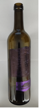
The following image of a wine bottle was used as a model to create the mesh. In principal, it is possible to build the geometry from a physical object by using functions like ImageMesh. To do so, a picture of the bottle must be taken. In order to avoid the curved opening and bottle bottom distorting the geometry, a special lens, a telecentric lens, needs to be used.
Here the geometry is created manually. The cross-sectional area of the bottle consists of two parts: a neck and a cavity. The neck is made of a rectangle primitive region, while the cavity is made of straight lines and curves.
To join both regions, they must first each be converted to a boundary element mesh and then BoundaryElementMeshUnion is used on them. This function is provided by the FEMAddOns paclet that can conveniently be installed with the resource function FEMAddOnsInstall.
Now, using the same setup as in the previous section, the model is solved.
To get the resonance frequency, the average pressure is computed over the cavity volume.
In addition to the experimental result, a comparison with a theoretical value is also possible.
Finally, the audio signal is analyzed to get the experimental resonance frequency. The audio used was recorded using AudioCapture, which uses an audio input device such as a built-in microphone.
The Audio object can be used directly in any computation.
Periodogram can be used to get a visualization of the squared magnitude of the discrete Fourier transform, the power spectrum, of the audio given in ![]() .
.
The peak shown in the spectrum represents the bottle's experimental resonance frequency, which is around 121 ![]() .
.
To get an exact value of the resonance frequency, the signal is converted into Fourier space. For this, PeriodogramArray can also be used.
To correctly visualize the power spectrum as a function of frequency, a list of frequencies needs to be created. This list of frequencies is based on the signal's sampling rate in the frequency space and the length of the audio.
This transform produces a mirror copy of the frequencies. These extra frequencies are the signal's negative frequency components and can be omitted.
Plotting the power spectrum as a function of frequency visualizes the signal's frequency components. Peaks correspond to a large power.
The power spectrum shows that the audio has a frequency component of around ![]() .
.
Three different values have been obtained for the resonant frequency: the simulation value, the measured value and the theoretical value.
Nomenclature
| Symbol | Description | Unit |
| ρ | density of a medium | [kg/m3] |
| c | speed of sound in a medium | [m/s] |
| p | sound pressure | [Pa] |
| ω | sound wave angular frequency | [rad/s] |
| f | sound wave frequency | [Hz] |
| rneck | radius of the neck | [m] |
| rcavity | radius of the cavity | [m] |
| l | length of the neck | [m] |
| lt | total length of the neck | [m] |
| Ω | computational domain | N/A |
| V | cavity volume | [m3] |
| S | neck cross-sectional area | [m2] |
| Lp | sound pressure level | [dB] |
References
1. Blackstock, D. T. (2001). Fundamentals of Physical Acoustics.
2. Li, L., Liu, Y., Zhang, F. and Sun, Z. (2017). "Several Explanations on the Theoretical Formula of Helmholtz Resonator." Advances in Engineering Software, 114, pp. 361–371.
3. Pierce, A. D. (2019). Acoustics: An Introduction to Its Physical Principles and Applications. Springer.
4. Rahim, R. A. and Johari, M. J. B. (2016). "Design and Simulation of MEMS Helmholtz Resonator for Acoustic Energy Harvester." 2016 International Conference on Computer and Communication Engineering (ICCCE).


