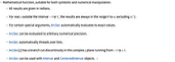
ArcSec[z]
给出复数
的反正割
.
ArcSec
ArcSec[z]
给出复数
的反正割
.
范例
打开所有单元 关闭所有单元基本范例 (5)
ArcSec[2]除以 Degree 已得到以度为单位的结果:
ArcSec[2] / Degree//FullSimplifyPlot[ArcSec[x], {x, -5, 5}]ComplexPlot3D[ArcSec[z], {z, -4 - 2I, 4 + 2I}, PlotLegends -> Automatic]在 Infinity 处的渐近展开:
Series[ArcSec[x], {x, ∞, 5}]Series[ArcSec[x], {x, 1, 3}, Assumptions -> x > 1]//Simplify范围 (41)
数值计算 (6)
ArcSec[5.0]N[ArcSec[5], 50]ArcSec[5.00000000000000000000000000000000000000000]ArcSec[0.5 + 2.3I]在高精度条件下高效计算 ArcSec:
ArcSec[5`500]//TimingArcSec[5`100000];//Timing用 Interval 和 CenteredInterval 对象计算最坏情况下的区间:
ArcSec[Interval[{2, 5}]]ArcSec[CenteredInterval[-3, 1 / 100]]ArcSec[CenteredInterval[2 + 3I, (1 + I) / 100]]或使用 Around 计算一般情况下的统计区间:
ArcSec[Around[(2/Sqrt[3]), 0.1]]ArcSec[{{Sqrt[2], -Sqrt[2]}, {0, -Sqrt[2]}}]或用 MatrixFunction 以矩阵形式计算 ArcSec 函数:
MatrixFunction[ArcSec[#]&, {{Sqrt[2], -Sqrt[2]}, {0, -Sqrt[2]}}]特殊值 (5)
ArcSec 在固定点上的值:
Table[ArcSec[n], {n, -2, 2}]ArcSec[(2/Sqrt[3])]ArcSec[Infinity]ArcSec[ComplexInfinity]ArcSec 的零点:
ArcSec[1]f[x_] := ArcSec[x] - (π/3);sol = Solve[f[x] == 0, x]xzero = x /. First[sol]Plot[f[x], {x, 1, 3}, Epilog -> Style[Point[{xzero, f[xzero]}], PointSize[Large], Red]]可视化 (3)
绘制 ArcSec 函数:
Plot[ArcSec[x], {x, -3, 3}]ComplexContourPlot[Re[ArcSec[z]], {z, -2 - 2I, 2 + 2I}, IconizedObject[«PlotOptions»]]ComplexContourPlot[Im[ArcSec[z]], {z, -2 - 2I, 2 + 2I}, IconizedObject[«PlotOptions»]]Table[PolarPlot[ArcSec[k ϕ], {ϕ, -5π, 5π}, Sequence[Frame -> True, PlotLabel -> "k=" <> ToString[k], PlotRange -> {{-2, 3}, {-3, 2}}]], {k, 1, 4}]函数属性 (10)
ArcSec 对区间
之外的所有实数有定义:
FunctionDomain[ArcSec[x], x]FunctionDomain[ArcSec[z], z, Complexes]ArcSec 的值域位于
到
:
FunctionRange[ArcSec[x], x, y]FunctionRange[ArcSec[z], z, y, Complexes]ArcSec 不是解析函数:
FunctionAnalytic[ArcSec[x], x]FunctionMeromorphic[ArcSec[x], x]ArcSec 在特定范围内是单调的:
FunctionMonotonicity[ArcSec[x], x]FunctionMonotonicity[{ArcSec[x], x ≤ -1 }, x]FunctionMonotonicity[{ArcSec[x], x ≥ 1}, x]Plot[ArcSec[x], {x, 1, 3}]ArcSec 是单射函数:
FunctionInjective[ArcSec[x], x]Plot[{ArcSec[x], 1 / 2}, {x, -5, 5}]ArcSec 不是满射函数:
FunctionSurjective[ArcSec[x], x]Plot[{ArcSec[x], π / 2}, {x, -5, 5}]ArcSec 在其实定义域上非负:
FunctionSign[{ArcSec[x], x ≤ -1 || x ≥ 1}, x]FunctionSingularities[ArcSec[x], x]FunctionDiscontinuities[ArcSec[x], x]ArcSec 既不凸,也不凹:
FunctionConvexity[ArcSec[x], x]TraditionalForm 格式:
ArcSec[x]//TraditionalForm微分 (3)
D[ArcSec[x], x]Table[D[ArcSec[x], {x, n}], {n, 1, 4}]//FullSimplifyPlot[Evaluate[%], {x, -3, 3}, PlotLegends -> {"First Derivative", "Second Derivative", "Third Derivative", "Fourth Derivative"}]D[ArcSec[x], {x, n}]积分 (3)
ArcSec 的不定积分:
Integrate[ArcSec[x], x]Integrate[ArcSec[x], {x, 1, 2}]Integrate[x ArcSec[x], x]Integrate[z ^ k ArcSec[z], z]级数展开式 (3)
使用 Series 求泰勒级数展开式:
Series[ArcSec[x], {x, 2, 4}]绘制 ArcSec 在
处的前三个近似式:
terms = Normal@Table[Series[ArcSec[x], {x, 2, m}], {m, 1, 3}];
Plot[{ArcSec[x], terms}, {x, 1, 3}, PlotRange -> {{1, 3}, {0, 2}}]Series[ArcSec[x], {x, 1, 1}]//FullSimplifySeries[ArcSec[x], {x, -1 / 2, 1}]ArcSec 可被应用于幂级数:
ArcSec[x + x ^ 2 + O[x, Infinity] ^ 4]函数恒等式和化简 (3)
函数表示 (5)
使用 ArcCos 表示:
ArcCos[(1/z)]//FullSimplifyInverseJacobiCD[(1/z), 0]//FullSimplifyInverseJacobiCN[(1/z), 0]//FullSimplify使用 Hypergeometric2F1 表示:
(π/2) - (Hypergeometric2F1[(1/2), (1/2), (3/2), (1/x^2)]/x)//FullSimplifyMeijerGReduce[ArcSec[x], x]Activate[%]//FullSimplifyArcSec 可被表示为 DifferentialRoot:
DifferentialRootReduce[ArcSec[x], x]应用 (3)
ArcSec 沿实轴延伸的分支切割:
Plot3D[Im[ArcSec[x + I y]], {x, -2, 2}, {y, -2, 2}]DSolve[Cos[y[x]] (1 - x Cos[y[x]]) + x Log[x] Sin[y[x]] Derivative[1][y][x] == 0, y[x], x]//Quiet使用 Parallelize 加快计算速度,可视化多个复三角函数:
$TrigFunctions = {Sin, Cos, Sec, Csc, Tan, Cot, ArcSin, ArcCos, ArcSec, ArcCsc, ArcTan, ArcCot};Parallelize@Table[Plot3D[Abs[f[x + I y]], {x, -2, 2}, {y, -2, 2}, MeshFunctions -> Function@@@{{{x, y, z}, Re[f[x + I y]]}, {{x, y, z}, Im[f[x + I y]]}}, MeshShading -> {{Orange, None}, {None, Green}}, PlotLabel -> f, Ticks -> None, ImageSize -> 100], {f, $TrigFunctions}]属性和关系 (5)
{ArcSec[Sec[z]], Sec[ArcSec[z]]}利用 PowerExpand 去掉 ArcSec 的多值性:
PowerExpand[%]Refine[ArcSec[Sec[z]], 0 < z < Pi / 2]利用 TrigToExp 以对数的形式表示:
ArcSec[z]//TrigToExp利用 ExpToTrig 反向变换:
ExpToTrig[%]ArcSec 给出以弧度为单位的角,ArcSecDegrees 给出相同的角,但以度为单位:
ArcSec[2]ArcSecDegrees[2]利用 FunctionExpand 将反三角函数的三角函数变换成代数函数:
FunctionExpand[Tan[5ArcSec[z]]]Simplify[%]Reduce[ArcSec[z] + ArcSec[z + 1] == Pi / 2, z]//Quiet技术笔记
-
▪
- 初等超越函数
相关指南
-
▪
- 三角函数
相关链接
历史
1988年引入 (1.0) | 在以下年份被更新:2021 (13.0)
文本
Wolfram Research (1988),ArcSec,Wolfram 语言函数,https://reference.wolfram.com/language/ref/ArcSec.html (更新于 2021 年).
CMS
Wolfram 语言. 1988. "ArcSec." Wolfram 语言与系统参考资料中心. Wolfram Research. 最新版本 2021. https://reference.wolfram.com/language/ref/ArcSec.html.
APA
Wolfram 语言. (1988). ArcSec. Wolfram 语言与系统参考资料中心. 追溯自 https://reference.wolfram.com/language/ref/ArcSec.html 年
BibTeX
@misc{reference.wolfram_2026_arcsec, author="Wolfram Research", title="{ArcSec}", year="2021", howpublished="\url{https://reference.wolfram.com/language/ref/ArcSec.html}", note=[Accessed: 09-August-2026]}
BibLaTeX
@online{reference.wolfram_2026_arcsec, organization={Wolfram Research}, title={ArcSec}, year={2021}, url={https://reference.wolfram.com/language/ref/ArcSec.html}, note=[Accessed: 09-August-2026]}