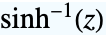


ArcSinh[z]
给出复数
的反双曲正弦函数
.
ArcSinh
ArcSinh[z]
给出复数
的反双曲正弦函数
.
背景
- ArcSinh 是反双曲正弦函数. 对实数
,ArcSinh[x] 表示满足
的双曲角度
且
. - ArcSinh 自动逐项作用于列表. 对某些特定变量值,ArcSinh 自动计算出精确值. 当给出精确数值表达式作为变量时,ArcSinh 可以算出任意精度的数值结果. 对包含 ArcSinh 的符号表达式,适用的操作运算有 FunctionExpand、TrigToExp、TrigExpand、Simplify 和 FullSimplify.
- 对复变量
,ArcSinh 的定义为
. ArcSinh[z] 在复平面
上有一个不连续的分支切割. - 与之相关的数学函数有 Sinh、ArcCosh 和 ArcSin.
范例
打开所有单元 关闭所有单元基本范例 (6)
ArcSinh[1.5]Plot[ArcSinh[x], {x, -10, 10}]ComplexPlot3D[ArcSinh[z], {z, -2 - 2I, 2 + 2I}, PlotLegends -> Automatic]Series[ArcSinh[x], {x, 0, 10}]在 Infinity 处的渐近展开:
Series[ArcSinh[x], {x, ∞, 3}]Series[ArcSinh[x], {x, I, 3}, Assumptions -> x > 1]范围 (45)
数值计算 (6)
ArcSinh[1.0]N[ArcSinh[1], 100]ArcSinh[1.000000000000000000000000000000000000000000000000000000]ArcSinh[1.5 + 0.7I]在高精度条件下高效计算 ArcSinh:
ArcSinh[1`500]//TimingArcSinh[1`100000];//Timing用 Interval 和 CenteredInterval 对象计算最坏情况下的区间:
ArcSinh[Interval[{-5 / 2, Sinh[2]}]]ArcSinh[CenteredInterval[3, 1 / 100]]ArcSinh[CenteredInterval[2 + 3I, (1 + I) / 100]]或使用 Around 计算一般情况下的统计区间:
ArcSinh[Around[.9, 0.1]]ArcSinh[{{I, I / Sqrt[2]}, {0, -I / Sqrt[2]}}]或用 MatrixFunction 以矩阵形式计算 ArcSinh 函数:
MatrixFunction[ArcSinh[#]&, {{I, I / Sqrt[2]}, {0, -I / Sqrt[2]}}]特殊值 (4)
ArcSinh 在固定点上的值:
Table[ArcSinh[(n /2)I], {n, -2, 2}]ArcSinh[Infinity]ArcSinh[ComplexInfinity]ArcSinh 的零点:
ArcSinh[0]f[x_] := ArcSinh[x] - Log[2];sol = Solve[f[x] == 0, x]xzero = x /. First[sol]Plot[f[x], {x, 0, 1}, Epilog -> Style[Point[{xzero, f[xzero]}], PointSize[Large], Red]]可视化 (3)
绘制 ArcSinh 函数:
Plot[ArcSinh[x], {x, -50, 50}]ComplexContourPlot[Re[ArcSinh[z]], {z, -3 - 3 I, 3 + 3 I}, IconizedObject[«PlotOptions»]]ComplexContourPlot[Im[ArcSinh[z]], {z, -3 - 3 I, 3 + 3 I}, IconizedObject[«PlotOptions»]]Table[PolarPlot[ArcSinh[k ϕ], {ϕ, -10π, 10π}, Frame -> True, Exclusions -> None, PlotLabel -> "k=" <> ToString[k], PlotRange -> {{-6, 6}, {-6, 6}}, FrameTicks -> {{{-6, -3, 0, 3, 6}, None}, {{-6, -3, 0, 3, 6}, None}}], {k, 1, 4}]函数属性 (12)
ArcSinh 是针对所有实数和复数定义的:
FunctionDomain[ArcSinh[x], x]FunctionDomain[ArcSinh[z], z, Complexes]ArcSinh 获取所有实数值:
FunctionRange[ArcSinh[x], x, y]FunctionRange[ArcSinh[z], z, y, Complexes]ArcSinh 是一个奇函数:
ArcSinh[-x]ArcSinh 具有镜像属性
:
FullSimplify[ArcSinh[Conjugate[z]] == Conjugate[ArcSinh[z]]]FunctionAnalytic[ArcSinh[x], x]FunctionAnalytic[ArcSinh[x], x, Complexes]FunctionMeromorphic[ArcSinh[x], x]ArcSinh 非递减:
FunctionMonotonicity[ArcSinh[x], x]ArcSinh 是单射函数:
FunctionInjective[ArcSinh[x], x]Plot[{ArcSinh[x], 1}, {x, -4, 4}]ArcSinh 是满射函数:
FunctionSurjective[ArcSinh[x], x]Plot[{ArcSinh[x], 10}, {x, -50000, 50000}, PlotRange -> {-12, 12}]ArcSinh 既不是非负,也不是非正:
FunctionSign[ArcSinh[x], x]ArcSinh 没有奇点和断点:
FunctionSingularities[ArcSinh[x], x]FunctionDiscontinuities[ArcSinh[x], x]ArcSinh 既不凸,也不凹:
FunctionConvexity[ArcSinh[x], x]TraditionalForm 格式输出:
ArcSinh[x]//TraditionalForm微分 (3)
D[ArcSinh[x], x]Table[D[ArcSinh[x], {x, n}], {n, 1, 4}]Plot[Evaluate[%], {x, -1, 1}, PlotLegends -> {"First Derivative", "Second Derivative", "Third Derivative", "Fourth Derivative"}]D[ArcSinh[x], {x, n}]积分 (3)
级数展开式 (4)
使用 Series 求泰勒级数展开式:
Series[ArcSinh[x], {x, 0, 7}]绘制 ArcSinh 在
处的前三个近似式:
terms = Normal@Table[Series[ArcSinh[x], {x, 0, m}], {m, 1, 5, 2}];
Plot[{ArcSinh[x], terms}, {x, -1.5, 1.5}, PlotRange -> {{-1.5, 1.5}, All}]ArcSinh 级数展开式的通项:
SeriesCoefficient[ArcSinh[x], {x, 0, n}]Series[ArcSinh[x], {x, I, 4}]Series[ArcSinh[x], {x, -2I, 4}]ArcSinh 可被应用于幂级数:
ArcSinh[Cos[x] + O[x] ^ 10]积分变换 (2)
用 FourierTransform 计算傅立叶变换:
FourierTransform[ArcSinh[t], t, ω]HankelTransform[ArcSinh[r], r, s]函数恒等式和化简 (3)
化简含有 ArcSinh 的表达式:
FullSimplify[Sinh[ArcSinh[x] + ArcSinh[y]]^4 - 2(2y^2 x^2 + x^2 + y^2)Sinh[ArcSinh[x] + ArcSinh[y]]^2 + (x^2 - y^2)^2]TrigToExp@ArcSinh[z]ExpToTrig[%]ComplexExpand[ArcSinh[x + I y]]函数表示 (5)
使用 ArcCsch 表示:
ArcCsch[1 / x]//FullSimplifyInverseJacobiCS[(1/z), 1]//FullSimplifyInverseJacobiSC[z, 1]使用 Hypergeometric2F1 表示:
x Hypergeometric2F1[(1/2), (1/2), (3/2), -x^2]MeijerGReduce[ArcSinh[x], x]Activate[%]ArcSinh 可被表示为 DifferentialRoot:
DifferentialRootReduce[ArcSinh[x], x]应用 (3)
Integrate[Sqrt[D[Sqrt[1 + t ^ 2], t] ^ 2 + 1], {t, 0, x}, Assumptions -> x > 0]N[% /. x -> 3, 20]DSolve[{(1 + x^2) y''[x] + x y'[x] == 1, y[0] == 0, y'[0] == 1}, y[x], x]u[x_, t_] := 2ArcSinh[JacobiCS[x - t, m]]FullSimplify[D[u[x, t], x, t] + Sinh[u[x, t]], JacobiNS[t - x, m] ^ 2 - JacobiCS[t - x, m] ^ 2 == 1]Plot3D[Evaluate[u[x, t] /. m -> 4 / 3], {x, -3, 2}, {t, 0, 5 / 2}]属性和关系 (4)
{ArcSinh[Sinh[z]], Sinh[ArcSinh[z]]}利用 PowerExpand 去掉 ArcSinh 的多值性:
PowerExpand[%]Refine[ArcSinh[Sinh[z]], z∈Reals]ArcSinh[z]//TrigToExpExpToTrig[%]Reduce[Sinh[x] == y, x]ArcSinh 是某些特殊函数的特殊情况:
x Hypergeometric2F1[1 / 2, 1 / 2, 3 / 2, -x ^ 2]可能存在的问题 (2)
技术笔记
-
▪
- 初等超越函数
相关指南
-
▪
- 双曲线函数 ▪
- 逆函数 ▪
- GPU 计算 ▪
- 初等函数 ▪
- NVIDIA GPU 计算 ▪
- Apple GPU 计算
历史
1988年引入 (1.0) | 在以下年份被更新:2021 (13.0)
文本
Wolfram Research (1988),ArcSinh,Wolfram 语言函数,https://reference.wolfram.com/language/ref/ArcSinh.html (更新于 2021 年).
CMS
Wolfram 语言. 1988. "ArcSinh." Wolfram 语言与系统参考资料中心. Wolfram Research. 最新版本 2021. https://reference.wolfram.com/language/ref/ArcSinh.html.
APA
Wolfram 语言. (1988). ArcSinh. Wolfram 语言与系统参考资料中心. 追溯自 https://reference.wolfram.com/language/ref/ArcSinh.html 年
BibTeX
@misc{reference.wolfram_2026_arcsinh, author="Wolfram Research", title="{ArcSinh}", year="2021", howpublished="\url{https://reference.wolfram.com/language/ref/ArcSinh.html}", note=[Accessed: 17-August-2026]}
BibLaTeX
@online{reference.wolfram_2026_arcsinh, organization={Wolfram Research}, title={ArcSinh}, year={2021}, url={https://reference.wolfram.com/language/ref/ArcSinh.html}, note=[Accessed: 17-August-2026]}