

AsymptoticExpectation[expr,xdist,aa0]
a0を中心とする expr の期待値についての漸近近似を,x が確率分布 dist に従うという仮定のもとに計算する.
AsymptoticExpectation[expr,{x1,x2,…}dist,aa0]
a0を中心とする expr の期待値についての漸近近似を,{x1,x2,…}が多変量分布 dist に従うという仮定のもとに計算する.
AsymptoticExpectation[expr,vars,{a,a0,n}]
漸近的な期待値を次数 n まで計算する.
AsymptoticExpectation
AsymptoticExpectation[expr,xdist,aa0]
a0を中心とする expr の期待値についての漸近近似を,x が確率分布 dist に従うという仮定のもとに計算する.
AsymptoticExpectation[expr,{x1,x2,…}dist,aa0]
a0を中心とする expr の期待値についての漸近近似を,{x1,x2,…}が多変量分布 dist に従うという仮定のもとに計算する.
AsymptoticExpectation[expr,vars,{a,a0,n}]
漸近的な期待値を次数 n まで計算する.
詳細とオプション
- 期待値の漸近近似は,平均その他の数量の値の推定に使われる.そのような用法の例として,大数の法則や1つあるいは複数のパラメータに依存する分布の研究が挙げられる.
- AsymptoticExpectation[expr,vars,aa0]は,expr の期待値のための任意の漸近展開において次数が最も高い項を計算する.SeriesTermGoalを使ってより多くの項を指定することができる.
- 中心 a0は,有限または無限の任意の実数または複素数でよい.
- 次数 n は漸近解の近似次数を指定する正の整数でなければならない.これは,多項式次数とは無関係である.
- 次は,使用可能なオプションである.
-
Assumptions $Assumptions パラメータについての仮定 GenerateConditions Automatic パラメータについての条件を含む答を生成するかどうか Method Automatic 使用するメソッド PerformanceGoal $PerformanceGoal パフォーマンスのどの面を最適化するか SeriesTermGoal Automatic 近似の項数
例題
すべて開く すべて閉じる例 (2)
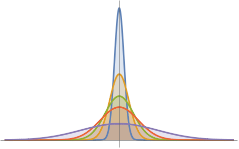
AsymptoticExpectation[2x ^ 2 + 3, xNormalDistribution[5a, E ^ a], a -> 0]Plot[Table[PDF[NormalDistribution[5a, E ^ a], x], {a, 0.1, 0.5, 0.1}]//Evaluate, {x, -3, 7}, PlotRange -> All, Filling -> Axis]AsymptoticExpectation[2x ^ 2 + 3, xNormalDistribution[5a, E ^ a], {a, 0, 2}]AsymptoticExpectation[E ^ (t x), xGammaDistribution[α, β], {t, 0, 3}]Table[Coefficient[%, t, k] * k!, {k, 1, 3}]//FactorTable[Moment[GammaDistribution[α, β], k], {k, 1, 3}]スコープ (9)
AsymptoticExpectation[(x - b) ^ 2 + 5UnitStep[x ^ 2 - 1], xNormalDistribution[0, b], {b, 1, 2}]AsymptoticExpectation[E ^ (d x) + 3, xPoissonDistribution[d], {d, 0, 5}]AsymptoticExpectation[x ^ b + 3y, {x, y}ProductDistribution[NormalDistribution[0, 1], ExponentialDistribution[b]], {b, 0, 2}]AsymptoticExpectation[2x + 3y + E ^ (b z), {x, y, z}MultinomialDistribution[10, {1 / 2, 1 / 3, 1 / 6}], {b, 0, 3}]TransformedDistributionについての漸近的期待値を計算する:
AsymptoticExpectation[x ^ 3, xTransformedDistribution[E ^ (-a y ^ 2), yExponentialDistribution[1]], {a, ∞, 4}]AsymptoticExpectation[E ^ (-x), xMixtureDistribution[{1, 2}, {NormalDistribution[2, a], NormalDistribution[4, a]}], {a, 0, 5}]AsymptoticExpectation[x, xParameterMixtureDistribution[ExponentialDistribution[λ], λBetaDistribution[α, α ^ 2]], α -> Infinity]AsymptoticExpectation[x^2 + E ^ x, xMarginalDistribution[DirichletDistribution[{1, 2, c}], 1], c -> 0]AsymptoticExpectation[E ^ (-b x ^ 2) + 2, xProbabilityDistribution[6 / 5(x ^ 2 + 2x), {x, 0, 1}], {b, ∞, 2}]アプリケーション (5)
AsymptoticExpectation[E ^ (-α x ^ 2), xExponentialDistribution[3], {α, 0, 3}, Assumptions -> α > 0]% /. {α -> 0.05}NExpectation[E ^ (-0.05 x ^ 2), xExponentialDistribution[3]]AsymptoticExpectation[x, xHoytDistribution[q, ω], {q, 0, 2}, Assumptions -> q > 0]dist = RiceDistribution[α, β];AsymptoticExpectation[(x - Mean[dist]) ^ 2, xdist, {α, 0, 3}, Assumptions -> α > 0]dist = RayleighDistribution[σ];AsymptoticExpectation[E ^ (t x), xdist, {t, 0, 3}]Table[Coefficient[%, t, k] * k!, {k, 1, 3}]//FactorTable[Moment[dist, k], {k, 1, 3}]Block[{n = 20, p = 1 / 2}, Show[
DiscretePlot[PDF[BinomialDistribution[n, p], k]//Evaluate, {k, n}, PlotRange -> All, PlotMarkers -> Automatic],
Plot[PDF[NormalDistribution[n p, Sqrt[n p - n p^2]], x], {x, -15, 25}, PlotStyle -> Thick]]]a1 = AsymptoticExpectation[E ^ (t x), xBinomialDistribution[n, p], {t, 0, 7}];対応する正規分布のモーメント母関数についての近似を計算する:
a2 = AsymptoticExpectation[E ^ (t x), xNormalDistribution[n p, Sqrt[n p - n p^2]], {t, 0, 7}];a1 /. {n -> 60., p -> 0.3}a2 /. {n -> 60., p -> 0.3}特性と関係 (4)
dist = UniformDistribution[{-1, 2}];AsymptoticExpectation[E ^ (a x), xdist, {a, 0, 3}]AsymptoticIntegrateを使って同じ結果を得る:
AsymptoticIntegrate[E ^ (a x) PDF[dist, x], {x, -∞, ∞}, {a, 0, 3}]dist = DiscreteUniformDistribution[{-2, 11}];AsymptoticExpectation[E ^ (a x), xdist, {a, 0, 3}]AsymptoticSumを使って同じ結果を得る:
AsymptoticSum[E ^ (a x) PDF[dist, x], {x, -∞, ∞}, {a, 0, 3}]NExpectationを使って期待値を数値で求める:
dist[b_] := ExponentialDistribution[b];AsymptoticExpectation[E ^ (-x ^ 2), xdist[b], {b, 0, 6}]% /. {b -> 0.14}NExpectation[E ^ (-x ^ 2), xdist[0.14]]Expectationを使って期待値を厳密値で求める:
dist[b_] := ExponentialDistribution[b];AsymptoticExpectation[E ^ (-x ^ 3), xdist[b], {b, 0, 6}]Expectation[E ^ (-x ^ 3), xdist[b]]Asymptoticを使って漸近近似を得る:
Asymptotic[%, {b, 0, 6}]関連するガイド
-
▪
- 漸近解析
テキスト
Wolfram Research (2020), AsymptoticExpectation, Wolfram言語関数, https://reference.wolfram.com/language/ref/AsymptoticExpectation.html.
CMS
Wolfram Language. 2020. "AsymptoticExpectation." Wolfram Language & System Documentation Center. Wolfram Research. https://reference.wolfram.com/language/ref/AsymptoticExpectation.html.
APA
Wolfram Language. (2020). AsymptoticExpectation. Wolfram Language & System Documentation Center. Retrieved from https://reference.wolfram.com/language/ref/AsymptoticExpectation.html
BibTeX
@misc{reference.wolfram_2026_asymptoticexpectation, author="Wolfram Research", title="{AsymptoticExpectation}", year="2020", howpublished="\url{https://reference.wolfram.com/language/ref/AsymptoticExpectation.html}", note=[Accessed: 08-August-2026]}
BibLaTeX
@online{reference.wolfram_2026_asymptoticexpectation, organization={Wolfram Research}, title={AsymptoticExpectation}, year={2020}, url={https://reference.wolfram.com/language/ref/AsymptoticExpectation.html}, note=[Accessed: 08-August-2026]}