AsymptoticSolve[eqn,yb,x->a]
{a,b}を通る方程式 eqn の解 y[x]の漸近近似を計算する.
AsymptoticSolve[eqn,{y},x->a]
方程式 eqn の解 y[x]の漸近近似を a の近くの x について計算する.
AsymptoticSolve[eqns,{y1,y2,…}{b1,b2,…},{x1,x2,…}{a1,a2,…}]
方程式系 eqns の解{y1[x1,x2,…],y2[x1,x2,…],…}の漸近近似を計算する.
AsymptoticSolve[eqns,…,{{x1,x2,…},{a1,a2,…},n}]
漸近近似を次数 n まで計算する.
実数値の引数についての実数値解のみを計算する.
AsymptoticSolve
AsymptoticSolve[eqn,yb,x->a]
{a,b}を通る方程式 eqn の解 y[x]の漸近近似を計算する.
AsymptoticSolve[eqn,{y},x->a]
方程式 eqn の解 y[x]の漸近近似を a の近くの x について計算する.
AsymptoticSolve[eqns,{y1,y2,…}{b1,b2,…},{x1,x2,…}{a1,a2,…}]
方程式系 eqns の解{y1[x1,x2,…],y2[x1,x2,…],…}の漸近近似を計算する.
AsymptoticSolve[eqns,…,{{x1,x2,…},{a1,a2,…},n}]
漸近近似を次数 n まで計算する.
実数値の引数についての実数値解のみを計算する.
詳細とオプション
- 漸近近似は,厳密解が求まらない問題を解いたり,計算,比較,解釈のより簡単な答を求めたりする際によく使われる.
- AsymptoticSolve[eqn,…,xa]は,eqn の漸近展開における最高次数の項を計算する.より多くの項が指定したければSeriesTermGoalを使うとよい.
- 漸近近似 yn[x] は,しばしば総和 yn[x]
αkϕk[x]として与えられる.ただし,{ϕ1[x],…,ϕn[x]}は xa のときの漸近尺度 ϕ1[x]≻ϕ2[x]≻⋯>ϕn[x]である.結果は,xa のとき,AsymptoticLess[y[x]-yn[x],ϕn[x],xa]または y[x]-yn[x]∈o[ϕn[x]]を満足する. - 次は,よく使われる漸近尺度である.
-

xa のときのテイラー(Taylor)スケール 

xa のときのローラン(Laurent)スケール 

x±∞のときのローランスケール 

xa のときのピュイゾー(Puiseux)スケール - 漸近近似を表すために使われる尺度は,問題から自動的に推測される.より珍しい尺度が含まれることも多い.
- 中心座標の a および b は,任意の,有限あるいは無限の実数あるいは複素数でよい.
- 次数 n は漸近解の近似次数を指定するもので,正の整数でなければならない.この次数は,多項式次数とは無関係である.
- 方程式系 eqns は方程式の任意の論理結合でよい.
- 次は,使用可能なオプションである.
-
Assumptions $Assumptions パラメータについての仮定 Direction Automatic x が a に近付く方向 GenerateConditions Automatic パラメータについての条件を含む答を生成するかどうか Method Automatic 使用するメソッド PerformanceGoal $PerformanceGoal パフォーマンスのどの局面について最適化するか SeriesTermGoal Automatic 漸近の項数 - 次は,Directionの可能な設定である.
-
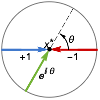
Reals または"TwoSided" 両実数方向から "FromAbove" または -1 上,つまりより大きい値から "FromBelow" または +1 下,つまりより小さい値から Complexes すべての複素方向から Exp[ θ]
の方向{dir1,…,dirn} 変数 xiに方向 diriを独立に使う - x*におけるDirectionExp[ θ]は,曲線の接線が極限点 x*に近付く方向を示す.
- 有限値の a についてのAutomatic設定は上からを意味する.
- 領域Realsが指定されると,x が指定されたDirectionから a に近付くときの解は実数値になる.
- 次は,GenerateConditionsの可能な設定である.
-
Automatic 一般的ではない条件のみ True すべての条件 False 条件なし None 条件が必要な場合には未評価で返す - PerformanceGoalの可能な設定には,$PerformanceGoal,"Quality","Speed"がある."Quality"設定のとき,AsymptoticSolveはより多くの問題を解いたりより簡単な結果を与えたりすることが多いが,より多くの時間とメモリが必要になる可能性がある.
例題
すべて開く すべて閉じる例 (5)
AsymptoticSolve[E^y - Cos[x y] + x == 0, {y, 0}, {x, 0, 7}]AsymptoticSolve[x y^4 - (x + 1) y^2 + x == 1, {y}, {x, 0, 3}]AsymptoticSolve[y ^ 3 + E ^ x y + x Log[x] == 0, y, x -> Infinity]AsymptoticSolve[x y^4 - (x + 1) y^2 + x == 1, {y}, {x, 0, 3}, Reals]AsymptoticSolve[x^2 - u (y + 1) == y^2 - v (x + 1) && u^2 - u (x + 1) == v^2 + v (y + 1), {{u, v}, {0, 0}}, {{x, y}, {0, 0}, 3}]スコープ (18)
2Dにおける一次元解 (8)
AsymptoticSolve[y ^ 3 - x y == 24, {y, 3}, {x, 1, 3}]asympt = First[y /. %];
exact[x_] := Last[y /. NSolve[y ^ 3 - x y == 24, y, Reals]]Plot[{asympt, exact[x]}, {x, -50, 50}, PlotStyle -> {Dashed, DotDashed}]f = Erf[x + y] - Log[1 + Sin[x y]];AsymptoticSolve[f == 0, {y, 0}, {x, 0, 3}]asympt = First[y /. %];
exact[x_] := y /. FindRoot[f, {y, asympt}]Plot[{asympt, exact[x]}, {x, -0.4, 0.4}, PlotStyle -> {Dashed, DotDashed}]AsymptoticSolve[y ^ 5 - x y + x ^ 2 == 0, {y, 0}, {x, 0, 5}]AsymptoticSolve[y ^ 5 - x y + x ^ 2 == 0, {y, 0}, {x, 0, 5}, Reals]AsymptoticSolve[y ^ 5 - x y + x ^ 2 == 0, {y, 0}, {x, 0, 5}, Reals, Direction -> "FromBelow"]AsymptoticSolve[Sin[x y] - y ^ 2 + x == 0, {y, 0}, {x, 0, 5}]AsymptoticSolve[Sin[y] - y ^ 2 + Cos[y] / Log[x] == 0, {y, 0}, {x, 0, 5}]AsymptoticSolve[x y ^ 4 + y ^ 2 - x ^ 2 y == 1, {y}, {x, 0, 3}]f = y ^ 5 - y / Sqrt[x] + x Log[x];AsymptoticSolve[f == 0, {y}, {x, Infinity, 3}, Reals]asympt = First[y /. %];
exact[x_] := First[y /. NSolve[f == 0, y, Reals]]Plot[{asympt, exact[x]}, {x, 1, 5}, PlotStyle -> {Dashed, DotDashed}]AsymptoticSolve[Sin[x y] - y Log[a + y] + x == 0, {y, 0}, {x, 0, 3}]AsymptoticSolve[y ^ 4 + a y ^ 3 + a x y - x ^ 2 + a x ^ 2 == 0, {y, Root[# ^ 4 + a # ^ 3&, 1]}, {x, 0, 3}]nDにおける一次元解 (5)
eqns = y ^ 3 - t x y == 21 && x ^ 2 - t ^ 2 y == 1;AsymptoticSolve[eqns, {{x, y}, {2, 3}}, {t, 1, 3}]asympt = First[{t, x, y} /. %];
exact = {t, x, y} /. Solve[eqns, {x, y}, Reals][[2]];ParametricPlot3D[{asympt, exact}, {t, 0, 2}, PlotStyle -> {Dashed, DotDashed}]eqns = Sin[t + x] + Cos[y] == t + 1 && Log[1 + x + y] - Sin[t] == 0;AsymptoticSolve[eqns, {{x, y}, {0, 0}}, {t, 0, 5}]asympt = First[{t, x, y} /. %];
exact[t_] := {t, x, y} /. FindRoot[eqns, {{x, asympt[[2]]}, {y, asympt[[3]]}}]ParametricPlot3D[{asympt, exact[t]}, {t, -0.9, 0.9}, PlotStyle -> {Dashed, DotDashed}]AsymptoticSolve[y ^ 2 - t x + t == 0 && x ^ 2 + t y == 0, {{x, y}, {0, 0}}, {t, 0, 2}]AsymptoticSolve[y ^ 2 - t x + t == 0 && x ^ 2 + t y == 0, {{x, y}, {0, 0}}, {t, 0, 2}, Reals]AsymptoticSolve[y ^ 2 - t x + t == 0 && x ^ 2 + t y == 0, {{x, y}, {0, 0}}, {t, 0, 2}, Reals, Direction -> "FromBelow"]AsymptoticSolve[y ^ 3 - t x y == 0 && x ^ 2 - t ^ 2 y == 1, {{x, y}}, {t, 0, 3}]AsymptoticSolve[{Sin[t + a x] + Cos[y] == t + 1, Log[1 + x + y] - Sin[t] == 0}, {{x, y}, {0, 0}}, {t, 0, 5}]nDにおけるより高次の次元の解 (5)
AsymptoticSolve[z ^ 5 - 2z ^ 3 + 2z + x ^ 2 - y == 0, {z, 0}, {{x, y}, {0, 0}, 5}]asympt = First[z /. %];
exact[x_, y_] := First[z /. NSolve[z ^ 5 - 2z ^ 3 + 2z + x ^ 2 - y == 0, z, Reals]];Plot3D[{asympt, exact[x, y]}, {x, -1, 1}, {y, -1, 1}, PlotLegends -> {"Asymptotic", "Exact"}, PlotStyle -> Opacity[0.7], BoxRatios -> 1]AsymptoticSolve[Exp[z + x - y] - Cos[x y] + x - y == 0, {z, 0}, {{x, y}, {0, 0}, 3}]asympt = First[z /. %];
exact[x_, y_] := z /. FindRoot[Exp[z + x - y] - Cos[x y] + x - y == 0, {z, asympt}]Plot3D[{asympt, exact[x, y]}, {x, -1, 1}, {y, -1, 1}, PlotLegends -> {"Asymptotic", "Exact"}, PlotStyle -> Opacity[0.7], BoxRatios -> 1]AsymptoticSolve[x ^ 2 - u (y + 1) == y ^ 2 - v (x + 1) + w && u ^ 2 - u (x + 1) == v ^ 2 + v (y + 1) - w && x + y == u + v + w, {{u, v, w}, {0, 0, 0}}, {{x, y}, {0, 0}, 3}]AsymptoticSolve[{Sin[u + x] + Cos[y] == v + 1, Log[1 + x + y] - u - Sin[u v] == 0}, {{u, v}, {0, 0}}, {{x, y}, {0, 0}, 3}]AsymptoticSolve[x ^ 2 - u == y ^ 2 - v(x + 1) - u ^ 2 && u ^ 2 - u(x + 1) == v ^ 2 + v, {{u, v}}, {{x, y}, {0, 0}, 2}]オプション (9)
Assumptions (1)
Assumptionsを使ってパラメータについての条件を指定する:
AsymptoticSolve[y ^ 3 - a y + x ^ 2y + x == 0, {y}, {x, 0, 3}, Reals, Assumptions -> a > 0]AsymptoticSolve[y ^ 3 - a y + x ^ 2y + x == 0, {y}, {x, 0, 3}, Reals, Assumptions -> a < 0]Direction (3)
デフォルトで,AsymptoticSolveは x が上から0に近付くときの有効な解を与える:
AsymptoticSolve[y ^ 3 + x ^ 2y + x == 0, {y}, {x, 0, 3}, Reals]AsymptoticSolve[y ^ 3 + x ^ 2y + x == 0, {y}, {x, 0, 3}, Reals, Direction -> "FromBelow"]AsymptoticSolve[y ^ 2 + E ^ (-2 / x) y + E ^ (-1 / x) == 0, {y, 0}, {x, 0, 5}, Direction -> "FromAbove"]AsymptoticSolve[y ^ 2 + E ^ (-2 / x) y + E ^ (-1 / x) == 0, {y, 0}, {x, 0, 5}, Direction -> "FromBelow"]AsymptoticSolve[x y ^ 7 + 2 x ^ 4 y ^ 6 + 3 x ^ 4 y ^ 3 - 2 x ^ 7 y ^ 2 - x ^ 10 == 0, {y, 0}, {x, 0, 3}, Reals, Direction -> E ^ (2 I Pi / 3)]GenerateConditions (3)
デフォルトで,AsymptoticSolveは結果を得るために仮定した条件を与える:
AsymptoticSolve[y ^ 3 + a y ^ 2 - x == 0, {y}, {x, 0, 3}, Reals]AsymptoticSolve[y ^ 3 + a y ^ 2 - x == 0, {y}, {x, 0, 3}, Reals, GenerateConditions -> False]AsymptoticSolve[y ^ 3 + a y ^ 2 - x == 0, {y}, {x, 0, 2}]GenerateConditions->Trueとすると,すべての条件が報告される:
AsymptoticSolve[y ^ 3 + a y ^ 2 - x == 0, {y}, {x, 0, 2}, GenerateConditions -> True]GenerateConditions->Noneのとき,AsymptoticSolveは一般的に有効な結果だけを返す:
AsymptoticSolve[y ^ 3 + a y ^ 2 - x == 0, {y}, {x, 0, 2}, GenerateConditions -> None]一般的ではない条件が必要な場合は,AsymptoticSolveは評価されずに返される:
AsymptoticSolve[y ^ 3 + a y ^ 2 - x == 0, {y}, {x, 0, 2}, Reals, GenerateConditions -> None]Method (1)
SeriesTermGoal (1)
デフォルトで,AsymptoticSolve[eqn,…,xa]は解の最高次の項を計算する:
AsymptoticSolve[Cos[x y] - Exp[y ^ 2 - 2x ^ 2] == 0, y -> 0, x -> 0]SeriesTermGoalを使ってより多くの項を得る:
AsymptoticSolve[Cos[x y] - Exp[y ^ 2 - 2x ^ 2] == 0, y -> 0, x -> 0, SeriesTermGoal -> 5]アプリケーション (12)
陰関数 (3)
方程式
は,それぞれ
近くの2つの異なる関数
を陰的に定義する.この2つの関数について
の近くの三次漸近近似を計算する:
AsymptoticSolve[y^2 == x, y, {x, 4, 3}]{yA1[x_], yA2[x_]} = y /. %;{yA1[4], yA2[4]}{yA1[4] ^ 2 == 4, yA2[4] ^ 2 == 4}ContourPlot[{y^2 == x, y == yA1[x], y == yA2[x]}, {x, -1, 6}, {y, -3, 3}, Epilog -> {PointSize[Large], Point[{{4, -2}, {4, 2}}]}]この場合,陰的に定義された2つの関数を厳密に解くのは簡単である:
{y1[x_], y2[x_]} = y /. Solve[y ^ 2 == x, y]AsymptoticSolveが返す2つの式は厳密解の級数である:
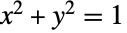
Series[yA1[x] - y1[x], {x, 4, 3}]//NormalSeries[yA2[x] - y2[x], {x, 4, 3}]//Normal{yR1[x_], yR2[x_]} = y /. AsymptoticSolve[y ^ 2 + x ^ 2 == 1, y, {x, 0, 2}]この近似は
のより大きいあるいはより小さい値についてのこれらの定点における円と非常に近い:
ContourPlot[{y ^ 2 + x ^ 2 == 1, y == yR1[x], y == yR2[x]}, {x, -3 / 2, 3 / 2}, {y, -3 / 2, 3 / 2}, Epilog -> {PointSize[Large], Point[{{0, 1}, {0, -1}}]}]{yS1[x_], yS2[x_]} = y /. AsymptoticSolve[y ^ 2 == 1 - x ^ 2, y, {x, 1, 2}]視覚的には,この近似は
の値についてしか定義されないように見える:
ContourPlot[{y ^ 2 + x ^ 2 == 1, y == yS1[x], y == yS2[x]}, {x, -3 / 2, 3 / 2}, {y, -3 / 2, 3 / 2}, Epilog -> {PointSize[Large], Point[{1, 0}]}]Plot[{Im[yS1[x]], Im[yS2[x]]}, {x, 0, 2}, PlotTheme -> {"Detailed", "DashedLines"}]AsymptoticSolve[y ^ 2 + x ^ 2 == 1, y, {x, 1, 2}, Reals]しかし,
のより小さい値に制限して純粋な実数式を求めることはできる:
AsymptoticSolve[y ^ 2 == 1 - x ^ 2, y, {x, 1, 2}, Reals, Direction -> "FromBelow"]曲線
は直線
と無限回交差する.垂直線テスト(任意の垂直線は曲線と1回しか交差せず,そのセクションと複数回交差する垂直線はない)をクリアする任意のセクションでは,関数は陰的に定義されている:
ContourPlot[{Sin[y] == x, x == 0}, {x, -1, 1}, {y, -3π, 3π}, PlotTheme -> "DashedLines"]AsymptoticSolve[Sin[y] == x, {y, 0}, {x, 0, 3}]これは,
の逆関数である
のテイラー級数にマッチすることに注意:
Series[ArcSin[x], {x, 0, 3}]AsymptoticSolve[Sin[y] == x, {y, Pi}, {x, 0, 3}]ContourPlot[{Sin[y] == x, x == 0, y == x + (x^3/6), y == π - x - (x^3/6)}, {x, -1.5, 1.5}, {y, -π, 2π}, IconizedObject[«ContourPlot options»]]摂動方程式 (2)
f = x ^ 3 - (6 + ϵ)x ^ 2 + (11 + ϵ)x - 6 + ϵ;AsymptoticSolve[f == 0, {x}, {ϵ, 0, 3}]asympt = x /. %;
exact = x /. Solve[f == 0, x];Plot[{asympt, exact}, {ϵ, 0, 0.5}, PlotStyle -> {Dashed, DotDashed}]f = Cos[x] - 1 + ϵ E ^ x;AsymptoticSolve[f == 0, {x, 0}, {ϵ, 0, 3}]asympt = x /. %;
exact[s_] := x /. FindRoot[f, {x, s}]Show[Plot[{#, exact[#]}, {ϵ, 0, 0.2}, PlotStyle -> {Dashed, DotDashed}]& /@ asympt, PlotRange -> All]方程式の級数解 (2)
f = Cos[x + y] - x + y - 1;D[f, y] /. {x -> 0, y -> 0}AsymptoticSolve[f == 0, {y, 0}, {x, 0, 5}]Series[f /. %[[1]], {x, 0, 5}]f = Sin[x + y + u + v] - u x + v y;
g = Exp[x - u] + Exp[y - v] - 2 Cos[x - v] + y - u;Det[D[{f, g}, {{x, y}}]] /. {x -> 0, y -> 0, u -> 0, v -> 0}AsymptoticSolve[f == 0 && g == 0, {{x, y}, {0, 0}}, {{u, v}, {0, 0}, 3}]Series[{f, g} /. %[[1]] /. {u -> t u, v -> t v}, {t, 0, 3}]曲線の漸近近似 (3)
f = y ^ 6 - 5x y ^ 4 + 3x ^ 2 y ^ 4 + 10x ^ 3 y ^ 2 + 3x ^ 4 y ^ 2 - x ^ 5 + x ^ 6;ls = AsymptoticSolve[f == 0, {y, 0}, {x, 0, 3}, Reals, Direction -> "FromBelow"]rs = AsymptoticSolve[f == 0, {y, 0}, {x, 0, 3}, Reals, Direction -> "FromAbove"]lp = ParametricPlot[Evaluate[{x, y} /. ls], {x, -1, 0}, PlotStyle -> {{Red, Dashed}}];rp = ParametricPlot[Evaluate[{x, y} /. rs], {x, 0, 1}, PlotStyle -> {{Red, Dashed}}];exact = ContourPlot[f == 0, {x, -1, 1}, {y, -1, 1}, PlotPoints -> 100];Show[{exact, lp, rp}]eqns = z ^ 2 - y ^ 2 + x y z + x ^ 2 z + x == 0 && x ^ 2 z ^ 2 + x y ^ 2 + y z + x y + x ^ 2 == 0;ls = AsymptoticSolve[eqns, {{y, z}, {0, 0}}, {x, 0, 3}, Reals, Direction -> "FromBelow"]rs = AsymptoticSolve[eqns, {{y, z}, {0, 0}}, {x, 0, 3}, Reals, Direction -> "FromAbove"]lasym = {x, y, z} /. ls;
rasym = {x, y, z} /. rs;
lp = ParametricPlot3D[lasym, {x, -0.3, 0}, PlotStyle -> {{Red, Dashed}}];
rp = ParametricPlot3D[rasym, {x, 0, 0.3}, PlotStyle -> {{Red, Dashed}}];nsol[s_] := {x, y, z} /. FindRoot[eqns, {{y, s[[2]]}, {z, s[[3]]}}]lpn = ParametricPlot3D[nsol /@ lasym, {x, -0.3, 0}, PlotStyle -> Blue];
rpn = ParametricPlot3D[nsol /@ rasym, {x, 0, 0.3}, PlotStyle -> Blue];Show[{lpn, rpn, lp, rp}, PlotRange -> All, BoxRatios -> 1]surf = ContourPlot3D[Evaluate[List@@eqns], {x, -0.3, 0.3}, {y, -0.6, 0.6}, {z, -0.6, 0.6}, Mesh -> None, ContourStyle -> {Directive[Orange, Opacity[0.3]], Directive[Yellow, Opacity[0.3]]}];Show[{surf, lpn, rpn, lp, rp}, PlotRange -> All, BoxRatios -> 1]AsymptoticSolve[x == r Cos[r ^ 2] && y == r Sin[r ^ 2], {{y, r}, {0, 0}}, {x, 0, 12}]asympt = First[y /. %];
ap = Plot[asympt, {x, 0, 1}, PlotStyle -> {Red, DotDashed}];
spiral = ParametricPlot[{r Cos[r ^ 2], r Sin[r ^ 2]}, {r, 0, 5}, PlotStyle -> Dashed];Show[{ap, spiral}, PlotRange -> All, AspectRatio -> Automatic]物理の問題の漸近解 (2)
平均近点角
についての離心近点角
のケプラー(Kepler)の方程式を解く:
AsymptoticSolve[M == Ε - e Sin[Ε], {Ε, 0}, {M, 0, 7}]asympt = First[Ε /. %] /. e -> 1 / 2;
exact[M_] := First[Ε /. Solve[M == Ε - 1 / 2Sin[Ε], Ε, Reals]//Quiet]Plot[{asympt, exact[M]}, {M, 0, 0.7}, PlotStyle -> {Dashed, DotDashed}]幅
,深さ
の一次元ボックス内の,質量
の粒子のエネルギーレベルを調べる.時間非依存シュレディンガー(Schrödinger)方程式のボックスの左側,ボックス内,ボックスの右側の解
,
,
は,以下で与えられる:
α = (Sqrt[2 m (V - Ε)]/ℏ);k = (Sqrt[2 m Ε]/ℏ);
Subscript[ψ, 1] = g Exp[α x];Subscript[ψ, 2] = a Sin[k x] + b Cos[k x];Subscript[ψ, 3] = h Exp[-α x];この解はボックスの境界上で連続的に微分可能でなければならない:
bconds = {(Subscript[ψ, 1] /. x -> -L / 2) == (Subscript[ψ, 2] /. x -> -L / 2), (Subscript[ψ, 2] /. x -> L / 2) == (Subscript[ψ, 3] /. x -> L / 2), (Subscript[∂, x]Subscript[ψ, 1] /. x -> -L / 2) == (Subscript[∂, x]Subscript[ψ, 2] /. x -> -L / 2), (Subscript[∂, x]Subscript[ψ, 2] /. x -> L / 2) == (Subscript[∂, x]Subscript[ψ, 3] /. x -> L / 2)}同次線形方程式は,その係数行列が特異のときは,非零の解を許す:
eqn = Det[CoefficientArrays[bconds, {a, b, g, h}][[2]]] == 0m = 1;L = 1; ℏ = 1;e1 = Ε /. Solve[(eqn /. V -> 1) && Ε > 0, Ε, Reals]AsymptoticSolve[eqn, {Ε, N[e1[[1]], 20]}, {V, 1, 5}]asympt = First[Ε /. %];
exact = Table[{V, Min[Ε /. Solve[eqn && Ε ≥ 1 / 1000, Ε, Reals]]}, {V, 1 / 4, 4, 1 / 4}];Show[{Plot[asympt, {V, 0.25, 4}], ListPlot[exact, PlotStyle -> Red]}]テキスト
Wolfram Research (2019), AsymptoticSolve, Wolfram言語関数, https://reference.wolfram.com/language/ref/AsymptoticSolve.html (2020年に更新).
CMS
Wolfram Language. 2019. "AsymptoticSolve." Wolfram Language & System Documentation Center. Wolfram Research. Last Modified 2020. https://reference.wolfram.com/language/ref/AsymptoticSolve.html.
APA
Wolfram Language. (2019). AsymptoticSolve. Wolfram Language & System Documentation Center. Retrieved from https://reference.wolfram.com/language/ref/AsymptoticSolve.html
BibTeX
@misc{reference.wolfram_2026_asymptoticsolve, author="Wolfram Research", title="{AsymptoticSolve}", year="2020", howpublished="\url{https://reference.wolfram.com/language/ref/AsymptoticSolve.html}", note=[Accessed: 14-September-2026]}
BibLaTeX
@online{reference.wolfram_2026_asymptoticsolve, organization={Wolfram Research}, title={AsymptoticSolve}, year={2020}, url={https://reference.wolfram.com/language/ref/AsymptoticSolve.html}, note=[Accessed: 14-September-2026]}