AsymptoticSolve[eqn,yb,x->a]
计算方程 eqn 的解 y[x] 经过 {a,b} 的渐近逼近.
AsymptoticSolve[eqn,{y},x->a]
计算方程 eqn 的解 y[x] 在 x 靠近 a 处的渐近逼近.
AsymptoticSolve[eqns,{y1,y2,…}{b1,b2,…},{x1,x2,…}{a1,a2,…}]
计算方程式系统 eqns 的解 {y1[x1,x2,…],y2[x1,x2,…],…} 的渐进逼近.
AsymptoticSolve[eqns,…,{{x1,x2,…},{a1,a2,…},n}]
计算 n 阶的渐近逼近.
仅计算实参数的实值解.
AsymptoticSolve
AsymptoticSolve[eqn,yb,x->a]
计算方程 eqn 的解 y[x] 经过 {a,b} 的渐近逼近.
AsymptoticSolve[eqn,{y},x->a]
计算方程 eqn 的解 y[x] 在 x 靠近 a 处的渐近逼近.
AsymptoticSolve[eqns,{y1,y2,…}{b1,b2,…},{x1,x2,…}{a1,a2,…}]
计算方程式系统 eqns 的解 {y1[x1,x2,…],y2[x1,x2,…],…} 的渐进逼近.
AsymptoticSolve[eqns,…,{{x1,x2,…},{a1,a2,…},n}]
计算 n 阶的渐近逼近.
仅计算实参数的实值解.
更多信息和选项
- 渐近逼近通常用于求解无法找到精确解的问题,或者为计算、比较和解释寻求更简单的答案.
- AsymptoticSolve[eqn,…,xa] 计算 eqn 的渐近展开式中的首项. 用 SeriesTermGoal 可指定计算更多的项.
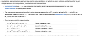
- 渐近逼近 yn[x] 常以和 yn[x]
αkϕk[x] 的形式给出,其中 {ϕ1[x],…,ϕn[x]} 是当 xa 时的渐近尺度 ϕ1[x]≻ϕ2[x]≻⋯>ϕn[x]. 则当 xa 时,结果满足 AsymptoticLess[y[x]-yn[x],ϕn[x],xa] 或 y[x]-yn[x]∈o[ϕn[x]]. - 常见的渐近尺度包括:
-

Taylor 尺度,当 xa 时 
Laurent 尺度,当 xa 时 

Laurent 尺度,当 x±∞ 时 

Puiseux 尺度,当 xa 时 - 用于表示渐近逼近的尺度是从问题中自动推断出来的,通常可以包含更多的奇异尺度.
- 中心坐标 a 和 b 可以为任意有限或无限大实数或复数.
- 阶数 n 必须为一个正整数,指定渐近解的近似阶数. 与多项式的次数无关.
- 方程组 eqns 可为方程的任意逻辑组合.
- 可以给出以下选项:
-
Assumptions $Assumptions 对参数的设定 Direction Automatic x 接近 a 的方向 GenerateConditions Automatic 是否给出与参数的条件有关的答案 Method Automatic 所用的方法 PerformanceGoal $PerformanceGoal 优化的目标 SeriesTermGoal Automatic 近似式的项数 - Direction 的可能设置包括:
-
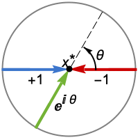
Reals 或 "TwoSided" 从两个实方向 "FromAbove" 或 -1 从上面或较大的值 "FromBelow" 或 +1 从下面或较小的值 Complexes 从所有复方向 Exp[ θ] 从方向 
{dir1,…,dirn} 对变量 xi 分别使用方向 diri - 在 x* 处的 DirectionExp[ θ] 表示接近极限点 x* 的曲线的方向切线.
- 对于 a 的有限值,Automatic 设置表示从上面接近.
- 如果指定了域 Reals,则当 x 从 Direction 逼近 a 时,解为实数.
- GenerateConditions 的可能设置包括:
-
Automatic 只给出非通用条件 True 所有条件 False 不给出条件 None 如果需要条件则不经计算直接返回 - PerformanceGoal 的可能设置包括 $PerformanceGoal、"Quality" 和 "Speed". 当设置为 "Quality" 时,AsymptoticSolve 通常可以解出更多的问题或者产生更简单的结果,但是可能会耗费更多的时间和内存.
范例
打开所有单元 关闭所有单元基本范例 (5)
AsymptoticSolve[E^y - Cos[x y] + x == 0, {y, 0}, {x, 0, 7}]AsymptoticSolve[x y^4 - (x + 1) y^2 + x == 1, {y}, {x, 0, 3}]AsymptoticSolve[y ^ 3 + E ^ x y + x Log[x] == 0, y, x -> Infinity]AsymptoticSolve[x y^4 - (x + 1) y^2 + x == 1, {y}, {x, 0, 3}, Reals]AsymptoticSolve[x^2 - u (y + 1) == y^2 - v (x + 1) && u^2 - u (x + 1) == v^2 + v (y + 1), {{u, v}, {0, 0}}, {{x, y}, {0, 0}, 3}]范围 (18)
二维空间中的一维解 (8)
AsymptoticSolve[y ^ 3 - x y == 24, {y, 3}, {x, 1, 3}]asympt = First[y /. %];
exact[x_] := Last[y /. NSolve[y ^ 3 - x y == 24, y, Reals]]Plot[{asympt, exact[x]}, {x, -50, 50}, PlotStyle -> {Dashed, DotDashed}]f = Erf[x + y] - Log[1 + Sin[x y]];AsymptoticSolve[f == 0, {y, 0}, {x, 0, 3}]asympt = First[y /. %];
exact[x_] := y /. FindRoot[f, {y, asympt}]Plot[{asympt, exact[x]}, {x, -0.4, 0.4}, PlotStyle -> {Dashed, DotDashed}]AsymptoticSolve[y ^ 5 - x y + x ^ 2 == 0, {y, 0}, {x, 0, 5}]AsymptoticSolve[y ^ 5 - x y + x ^ 2 == 0, {y, 0}, {x, 0, 5}, Reals]AsymptoticSolve[y ^ 5 - x y + x ^ 2 == 0, {y, 0}, {x, 0, 5}, Reals, Direction -> "FromBelow"]AsymptoticSolve[Sin[x y] - y ^ 2 + x == 0, {y, 0}, {x, 0, 5}]AsymptoticSolve[Sin[y] - y ^ 2 + Cos[y] / Log[x] == 0, {y, 0}, {x, 0, 5}]AsymptoticSolve[x y ^ 4 + y ^ 2 - x ^ 2 y == 1, {y}, {x, 0, 3}]f = y ^ 5 - y / Sqrt[x] + x Log[x];AsymptoticSolve[f == 0, {y}, {x, Infinity, 3}, Reals]asympt = First[y /. %];
exact[x_] := First[y /. NSolve[f == 0, y, Reals]]Plot[{asympt, exact[x]}, {x, 1, 5}, PlotStyle -> {Dashed, DotDashed}]AsymptoticSolve[Sin[x y] - y Log[a + y] + x == 0, {y, 0}, {x, 0, 3}]AsymptoticSolve[y ^ 4 + a y ^ 3 + a x y - x ^ 2 + a x ^ 2 == 0, {y, Root[# ^ 4 + a # ^ 3&, 1]}, {x, 0, 3}]n (5) 维空间中的一维解
eqns = y ^ 3 - t x y == 21 && x ^ 2 - t ^ 2 y == 1;AsymptoticSolve[eqns, {{x, y}, {2, 3}}, {t, 1, 3}]asympt = First[{t, x, y} /. %];
exact = {t, x, y} /. Solve[eqns, {x, y}, Reals][[2]];ParametricPlot3D[{asympt, exact}, {t, 0, 2}, PlotStyle -> {Dashed, DotDashed}]eqns = Sin[t + x] + Cos[y] == t + 1 && Log[1 + x + y] - Sin[t] == 0;AsymptoticSolve[eqns, {{x, y}, {0, 0}}, {t, 0, 5}]asympt = First[{t, x, y} /. %];
exact[t_] := {t, x, y} /. FindRoot[eqns, {{x, asympt[[2]]}, {y, asympt[[3]]}}]ParametricPlot3D[{asympt, exact[t]}, {t, -0.9, 0.9}, PlotStyle -> {Dashed, DotDashed}]AsymptoticSolve[y ^ 2 - t x + t == 0 && x ^ 2 + t y == 0, {{x, y}, {0, 0}}, {t, 0, 2}]AsymptoticSolve[y ^ 2 - t x + t == 0 && x ^ 2 + t y == 0, {{x, y}, {0, 0}}, {t, 0, 2}, Reals]AsymptoticSolve[y ^ 2 - t x + t == 0 && x ^ 2 + t y == 0, {{x, y}, {0, 0}}, {t, 0, 2}, Reals, Direction -> "FromBelow"]AsymptoticSolve[y ^ 3 - t x y == 0 && x ^ 2 - t ^ 2 y == 1, {{x, y}}, {t, 0, 3}]AsymptoticSolve[{Sin[t + a x] + Cos[y] == t + 1, Log[1 + x + y] - Sin[t] == 0}, {{x, y}, {0, 0}}, {t, 0, 5}]n (5) 维空间中的高维解
AsymptoticSolve[z ^ 5 - 2z ^ 3 + 2z + x ^ 2 - y == 0, {z, 0}, {{x, y}, {0, 0}, 5}]asympt = First[z /. %];
exact[x_, y_] := First[z /. NSolve[z ^ 5 - 2z ^ 3 + 2z + x ^ 2 - y == 0, z, Reals]];Plot3D[{asympt, exact[x, y]}, {x, -1, 1}, {y, -1, 1}, PlotLegends -> {"Asymptotic", "Exact"}, PlotStyle -> Opacity[0.7], BoxRatios -> 1]AsymptoticSolve[Exp[z + x - y] - Cos[x y] + x - y == 0, {z, 0}, {{x, y}, {0, 0}, 3}]asympt = First[z /. %];
exact[x_, y_] := z /. FindRoot[Exp[z + x - y] - Cos[x y] + x - y == 0, {z, asympt}]Plot3D[{asympt, exact[x, y]}, {x, -1, 1}, {y, -1, 1}, PlotLegends -> {"Asymptotic", "Exact"}, PlotStyle -> Opacity[0.7], BoxRatios -> 1]AsymptoticSolve[x ^ 2 - u (y + 1) == y ^ 2 - v (x + 1) + w && u ^ 2 - u (x + 1) == v ^ 2 + v (y + 1) - w && x + y == u + v + w, {{u, v, w}, {0, 0, 0}}, {{x, y}, {0, 0}, 3}]AsymptoticSolve[{Sin[u + x] + Cos[y] == v + 1, Log[1 + x + y] - u - Sin[u v] == 0}, {{u, v}, {0, 0}}, {{x, y}, {0, 0}, 3}]AsymptoticSolve[x ^ 2 - u == y ^ 2 - v(x + 1) - u ^ 2 && u ^ 2 - u(x + 1) == v ^ 2 + v, {{u, v}}, {{x, y}, {0, 0}, 2}]选项 (9)
Assumptions (1)
用 Assumptions 为参数指定条件:
AsymptoticSolve[y ^ 3 - a y + x ^ 2y + x == 0, {y}, {x, 0, 3}, Reals, Assumptions -> a > 0]AsymptoticSolve[y ^ 3 - a y + x ^ 2y + x == 0, {y}, {x, 0, 3}, Reals, Assumptions -> a < 0]Direction (3)
默认情况下,AsymptoticSolve 当 x 从上面逼近 0 时的解:
AsymptoticSolve[y ^ 3 + x ^ 2y + x == 0, {y}, {x, 0, 3}, Reals]AsymptoticSolve[y ^ 3 + x ^ 2y + x == 0, {y}, {x, 0, 3}, Reals, Direction -> "FromBelow"]AsymptoticSolve[y ^ 2 + E ^ (-2 / x) y + E ^ (-1 / x) == 0, {y, 0}, {x, 0, 5}, Direction -> "FromAbove"]AsymptoticSolve[y ^ 2 + E ^ (-2 / x) y + E ^ (-1 / x) == 0, {y, 0}, {x, 0, 5}, Direction -> "FromBelow"]AsymptoticSolve[x y ^ 7 + 2 x ^ 4 y ^ 6 + 3 x ^ 4 y ^ 3 - 2 x ^ 7 y ^ 2 - x ^ 10 == 0, {y, 0}, {x, 0, 3}, Reals, Direction -> E ^ (2 I Pi / 3)]GenerateConditions (3)
默认情况下,AsymptoticSolve 对能给出结果的情况产生条件:
AsymptoticSolve[y ^ 3 + a y ^ 2 - x == 0, {y}, {x, 0, 3}, Reals]AsymptoticSolve[y ^ 3 + a y ^ 2 - x == 0, {y}, {x, 0, 3}, Reals, GenerateConditions -> False]AsymptoticSolve[y ^ 3 + a y ^ 2 - x == 0, {y}, {x, 0, 2}]当设置为 GenerateConditions->True 时,所有条件都要报告:
AsymptoticSolve[y ^ 3 + a y ^ 2 - x == 0, {y}, {x, 0, 2}, GenerateConditions -> True]当设置为 GenerateConditions->None 时,AsymptoticSolve 只返回通常情况下有效的解:
AsymptoticSolve[y ^ 3 + a y ^ 2 - x == 0, {y}, {x, 0, 2}, GenerateConditions -> None]如果需要非通用条件,AsymptoticSolve 不执行任何计算,直接返回:
AsymptoticSolve[y ^ 3 + a y ^ 2 - x == 0, {y}, {x, 0, 2}, Reals, GenerateConditions -> None]Method (1)
SeriesTermGoal (1)
默认情况下,AsymptoticSolve[eqn,…,xa] 计算解的首项:
AsymptoticSolve[Cos[x y] - Exp[y ^ 2 - 2x ^ 2] == 0, y -> 0, x -> 0]用 SeriesTermGoal 获得更多项:
AsymptoticSolve[Cos[x y] - Exp[y ^ 2 - 2x ^ 2] == 0, y -> 0, x -> 0, SeriesTermGoal -> 5]应用 (12)
隐函数 (3)
方程
隐式定义了
附近的两个不同的函数
. 计算这两个函数在
附近的三阶渐近近似:
AsymptoticSolve[y^2 == x, y, {x, 4, 3}]{yA1[x_], yA2[x_]} = y /. %;{yA1[4], yA2[4]}{yA1[4] ^ 2 == 4, yA2[4] ^ 2 == 4}ContourPlot[{y^2 == x, y == yA1[x], y == yA2[x]}, {x, -1, 6}, {y, -3, 3}, Epilog -> {PointSize[Large], Point[{{4, -2}, {4, 2}}]}]{y1[x_], y2[x_]} = y /. Solve[y ^ 2 == x, y]AsymptoticSolve 返回的两个表达式是精确解的级数:
Series[yA1[x] - y1[x], {x, 4, 3}]//NormalSeries[yA2[x] - y2[x], {x, 4, 3}]//Normal{yR1[x_], yR2[x_]} = y /. AsymptoticSolve[y ^ 2 + x ^ 2 == 1, y, {x, 0, 2}]ContourPlot[{y ^ 2 + x ^ 2 == 1, y == yR1[x], y == yR2[x]}, {x, -3 / 2, 3 / 2}, {y, -3 / 2, 3 / 2}, Epilog -> {PointSize[Large], Point[{{0, 1}, {0, -1}}]}]{yS1[x_], yS2[x_]} = y /. AsymptoticSolve[y ^ 2 == 1 - x ^ 2, y, {x, 1, 2}]ContourPlot[{y ^ 2 + x ^ 2 == 1, y == yS1[x], y == yS2[x]}, {x, -3 / 2, 3 / 2}, {y, -3 / 2, 3 / 2}, Epilog -> {PointSize[Large], Point[{1, 0}]}]Plot[{Im[yS1[x]], Im[yS2[x]]}, {x, 0, 2}, PlotTheme -> {"Detailed", "DashedLines"}]AsymptoticSolve[y ^ 2 + x ^ 2 == 1, y, {x, 1, 2}, Reals]AsymptoticSolve[y ^ 2 == 1 - x ^ 2, y, {x, 1, 2}, Reals, Direction -> "FromBelow"]曲线
无限多次穿过直线
. 在通过垂直线测试(任何垂直线只与曲线相交一次;没有垂直线多次与该部分相交)的部分,隐式定义了一个函数:
ContourPlot[{Sin[y] == x, x == 0}, {x, -1, 1}, {y, -3π, 3π}, PlotTheme -> "DashedLines"]AsymptoticSolve[Sin[y] == x, {y, 0}, {x, 0, 3}]Series[ArcSin[x], {x, 0, 3}]AsymptoticSolve[Sin[y] == x, {y, Pi}, {x, 0, 3}]ContourPlot[{Sin[y] == x, x == 0, y == x + (x^3/6), y == π - x - (x^3/6)}, {x, -1.5, 1.5}, {y, -π, 2π}, IconizedObject[«ContourPlot options»]]摄动方程 (2)
f = x ^ 3 - (6 + ϵ)x ^ 2 + (11 + ϵ)x - 6 + ϵ;AsymptoticSolve[f == 0, {x}, {ϵ, 0, 3}]asympt = x /. %;
exact = x /. Solve[f == 0, x];Plot[{asympt, exact}, {ϵ, 0, 0.5}, PlotStyle -> {Dashed, DotDashed}]f = Cos[x] - 1 + ϵ E ^ x;AsymptoticSolve[f == 0, {x, 0}, {ϵ, 0, 3}]asympt = x /. %;
exact[s_] := x /. FindRoot[f, {x, s}]Show[Plot[{#, exact[#]}, {ϵ, 0, 0.2}, PlotStyle -> {Dashed, DotDashed}]& /@ asympt, PlotRange -> All]方程的级数解 (2)
f = Cos[x + y] - x + y - 1;D[f, y] /. {x -> 0, y -> 0}AsymptoticSolve[f == 0, {y, 0}, {x, 0, 5}]Series[f /. %[[1]], {x, 0, 5}]f = Sin[x + y + u + v] - u x + v y;
g = Exp[x - u] + Exp[y - v] - 2 Cos[x - v] + y - u;Det[D[{f, g}, {{x, y}}]] /. {x -> 0, y -> 0, u -> 0, v -> 0}AsymptoticSolve[f == 0 && g == 0, {{x, y}, {0, 0}}, {{u, v}, {0, 0}, 3}]Series[{f, g} /. %[[1]] /. {u -> t u, v -> t v}, {t, 0, 3}]曲线的渐近近似 (3)
f = y ^ 6 - 5x y ^ 4 + 3x ^ 2 y ^ 4 + 10x ^ 3 y ^ 2 + 3x ^ 4 y ^ 2 - x ^ 5 + x ^ 6;ls = AsymptoticSolve[f == 0, {y, 0}, {x, 0, 3}, Reals, Direction -> "FromBelow"]rs = AsymptoticSolve[f == 0, {y, 0}, {x, 0, 3}, Reals, Direction -> "FromAbove"]lp = ParametricPlot[Evaluate[{x, y} /. ls], {x, -1, 0}, PlotStyle -> {{Red, Dashed}}];rp = ParametricPlot[Evaluate[{x, y} /. rs], {x, 0, 1}, PlotStyle -> {{Red, Dashed}}];exact = ContourPlot[f == 0, {x, -1, 1}, {y, -1, 1}, PlotPoints -> 100];Show[{exact, lp, rp}]eqns = z ^ 2 - y ^ 2 + x y z + x ^ 2 z + x == 0 && x ^ 2 z ^ 2 + x y ^ 2 + y z + x y + x ^ 2 == 0;ls = AsymptoticSolve[eqns, {{y, z}, {0, 0}}, {x, 0, 3}, Reals, Direction -> "FromBelow"]rs = AsymptoticSolve[eqns, {{y, z}, {0, 0}}, {x, 0, 3}, Reals, Direction -> "FromAbove"]lasym = {x, y, z} /. ls;
rasym = {x, y, z} /. rs;
lp = ParametricPlot3D[lasym, {x, -0.3, 0}, PlotStyle -> {{Red, Dashed}}];
rp = ParametricPlot3D[rasym, {x, 0, 0.3}, PlotStyle -> {{Red, Dashed}}];nsol[s_] := {x, y, z} /. FindRoot[eqns, {{y, s[[2]]}, {z, s[[3]]}}]lpn = ParametricPlot3D[nsol /@ lasym, {x, -0.3, 0}, PlotStyle -> Blue];
rpn = ParametricPlot3D[nsol /@ rasym, {x, 0, 0.3}, PlotStyle -> Blue];Show[{lpn, rpn, lp, rp}, PlotRange -> All, BoxRatios -> 1]surf = ContourPlot3D[Evaluate[List@@eqns], {x, -0.3, 0.3}, {y, -0.6, 0.6}, {z, -0.6, 0.6}, Mesh -> None, ContourStyle -> {Directive[Orange, Opacity[0.3]], Directive[Yellow, Opacity[0.3]]}];Show[{surf, lpn, rpn, lp, rp}, PlotRange -> All, BoxRatios -> 1]AsymptoticSolve[x == r Cos[r ^ 2] && y == r Sin[r ^ 2], {{y, r}, {0, 0}}, {x, 0, 12}]asympt = First[y /. %];
ap = Plot[asympt, {x, 0, 1}, PlotStyle -> {Red, DotDashed}];
spiral = ParametricPlot[{r Cos[r ^ 2], r Sin[r ^ 2]}, {r, 0, 5}, PlotStyle -> Dashed];Show[{ap, spiral}, PlotRange -> All, AspectRatio -> Automatic]物理问题的渐近解 (2)
AsymptoticSolve[M == Ε - e Sin[Ε], {Ε, 0}, {M, 0, 7}]asympt = First[Ε /. %] /. e -> 1 / 2;
exact[M_] := First[Ε /. Solve[M == Ε - 1 / 2Sin[Ε], Ε, Reals]//Quiet]Plot[{asympt, exact[M]}, {M, 0, 0.7}, PlotStyle -> {Dashed, DotDashed}]研究宽度为
、深度为
的一维盒中质量为
的粒子的能级. 下面给出了不含时薛定谔方程在盒子左边的解、盒子中的解和盒子右边的解
、
和
:
α = (Sqrt[2 m (V - Ε)]/ℏ);k = (Sqrt[2 m Ε]/ℏ);
Subscript[ψ, 1] = g Exp[α x];Subscript[ψ, 2] = a Sin[k x] + b Cos[k x];Subscript[ψ, 3] = h Exp[-α x];bconds = {(Subscript[ψ, 1] /. x -> -L / 2) == (Subscript[ψ, 2] /. x -> -L / 2), (Subscript[ψ, 2] /. x -> L / 2) == (Subscript[ψ, 3] /. x -> L / 2), (Subscript[∂, x]Subscript[ψ, 1] /. x -> -L / 2) == (Subscript[∂, x]Subscript[ψ, 2] /. x -> -L / 2), (Subscript[∂, x]Subscript[ψ, 2] /. x -> L / 2) == (Subscript[∂, x]Subscript[ψ, 3] /. x -> L / 2)}eqn = Det[CoefficientArrays[bconds, {a, b, g, h}][[2]]] == 0m = 1;L = 1; ℏ = 1;e1 = Ε /. Solve[(eqn /. V -> 1) && Ε > 0, Ε, Reals]AsymptoticSolve[eqn, {Ε, N[e1[[1]], 20]}, {V, 1, 5}]asympt = First[Ε /. %];
exact = Table[{V, Min[Ε /. Solve[eqn && Ε ≥ 1 / 1000, Ε, Reals]]}, {V, 1 / 4, 4, 1 / 4}];Show[{Plot[asympt, {V, 0.25, 4}], ListPlot[exact, PlotStyle -> Red]}]文本
Wolfram Research (2019),AsymptoticSolve,Wolfram 语言函数,https://reference.wolfram.com/language/ref/AsymptoticSolve.html (更新于 2020 年).
CMS
Wolfram 语言. 2019. "AsymptoticSolve." Wolfram 语言与系统参考资料中心. Wolfram Research. 最新版本 2020. https://reference.wolfram.com/language/ref/AsymptoticSolve.html.
APA
Wolfram 语言. (2019). AsymptoticSolve. Wolfram 语言与系统参考资料中心. 追溯自 https://reference.wolfram.com/language/ref/AsymptoticSolve.html 年
BibTeX
@misc{reference.wolfram_2026_asymptoticsolve, author="Wolfram Research", title="{AsymptoticSolve}", year="2020", howpublished="\url{https://reference.wolfram.com/language/ref/AsymptoticSolve.html}", note=[Accessed: 08-August-2026]}
BibLaTeX
@online{reference.wolfram_2026_asymptoticsolve, organization={Wolfram Research}, title={AsymptoticSolve}, year={2020}, url={https://reference.wolfram.com/language/ref/AsymptoticSolve.html}, note=[Accessed: 08-August-2026]}