Blend
詳細
- Blendは,色付きの光源あるいは発色表示に適する加法混色を実装する.
- Blend[{col1,…,coln},{u1,…,un}]では,ui は合計が1になるように正規化される. »
- Blend[{col1,col2,…}]は,すべての coliを同じ割合で合成する.
- Blend[{image1,image2},x]では,image1 と image2 の次元が異なる場合は,次元の線形補間が使われる.
- Blend[{image,col},x]は,image のすべての画素を色 col と合成する.
- Blend[{image1,col1,…,coln,image2},x]では,coli は,次元が image1の次元と image2の次元の線形補間による画像であると解釈される.
例題
すべて開く すべて閉じる例 (4)
Blend[{Red, Blue}, 1 / 3]Graphics[Table[{Blend[{Red, Blue}, x], Disk[{8x, 0}]}, {x, 0, 1, 1 / 8}]]Plot3D[Sin[x + y ^ 2], {x, -3, 3}, {y, -2, 2}, ColorFunction -> (Blend[{Yellow, Purple}, #3]&)]Blend[{[image], Magenta}]スコープ (12)
色 (6)
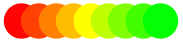
Blend[{Red, Green}]Graphics[{Blend[{Red, Green}], Disk[]}]Graphics[Table[{Blend[{Red, Green}, x], Disk[{8x, 0}]}, {x, 0, 1, 1 / 8}]]Blend[{RGBColor[1, 0, 0, 1], RGBColor[0, 1, 0, 0]}]Graphics[Table[{Blend[{RGBColor[1, 0, 0, 1], RGBColor[0, 1, 0, 0]}, x], Disk[{8x, 0}]}, {x, 0, 1, 1 / 8}]]Graphics[Table[{Blend[{Red, Yellow, Green}, x], Disk[{8x, 0}]}, {x, 0, 1, 1 / 8}]]Graphics[Table[{Blend[{{1, Red}, {3, Yellow}, {10, Green}}, x], Disk[{x, 0}]}, {x, 1, 10}]]Blend[{RGBColor[1, 0, 0], RGBColor[0, 1, 0], RGBColor[0, 0, 1]}]Blend[{RGBColor[1, 0, 0], RGBColor[0, 1, 0], RGBColor[0, 0, 1]}, {1 / 8, 1 / 2, 3 / 8}]ParametricPlot[{x, y}, {x, 0, 1}, {y, 0, 1 - x}, ColorFunction -> Function[{x, y}, Blend[{Red, Green, Blue}, {x, y, 1 - x - y}]]]画像 (6)
Blend[{[image], Yellow}]Blend[{[image], Yellow}, .2]Blend[{[image], [image]}]Blend[{[image], [image]}]Blend[{[image], [image]}]Blend[{\!\(\*Graphics3DBox[«8»]\), \!\(\*Graphics3DBox[«8»]\)}]アプリケーション (2)
Blendを使って基調色からColorFunctionを構成する:
Plot[1 / x Sin[x ^ 2], {x, 0, 6}, ColorFunction -> (Blend[{LightBlue, Blue}, #2]&), PlotStyle -> Thick]Plot3D[ x y / (x ^ 2 + y ^ 2), {x, -2, 2}, {y, -2, 2}, RegionFunction -> Function[{x, y, z}, x^2 + y^2 > 0.1], ColorFunction -> (Blend[{Lighter[Yellow, .8], Orange, Red}, #3]&), Mesh -> None]ContourPlot3D[x ^ 2 + y ^ 2 - z ^ 4 + z ^ 5 == 0, {x, -1, 1}, {y, -1, 1}, {z, -1, 1}, ColorFunction -> (Blend[{Cyan, Magenta, Yellow}, {#1, #2, #3}]&), Mesh -> None, ContourStyle -> Opacity[0.7]]Blend[{[image], [image], [image], [image], [image]}]特性と関係 (7)
Blend[{Red, Green, Blue}, {1, 2, 3}]%//InputFormGraphics[Raster[{Range[100] / 100}, ColorFunction -> (Blend[{{0, Red}, {1, Green}, {2 / 3, Yellow}, {1 / 3, Blue}}, #]&)], AspectRatio -> .3]色が同じ色空間を使って指定された場合,その空間は補間に用いられる:
Column[Labeled[ArrayPlot[{Table[Blend[ColorConvert[{Blue, Red}, #], n], {n, 0, 1, .01}]}, AspectRatio -> .25], #]& /@ {RGBColor, Hue, XYZColor, LCHColor}]色が異なる色空間で指定された場合,補間はRGB空間で行われる:
ArrayPlot[{Table[Blend[{Red, Hue[2 / 3]}, n], {n, 0, 1, .01}]}, AspectRatio -> .25]{Lighter[Blue, 1 / 3], Blend[{Blue, White}, 1 / 3]}{Darker[Blue, 1 / 3], Blend[{Blue, Black}, 1 / 3]}ColorDataは"Gradients"と呼ばれる多くの予め定義されたBlendされた(混合)色を含んでいる:
ColorData["Gradients"]//ShortColorData["TemperatureMap", "Image"]DensityPlot[x, {x, 0, 1}, {y, 0, 1}, ColorFunction -> (ColorData["SunsetColors"][#]&)]DensityPlot[x, {x, 0, 1}, {y, 0, 1}, ColorFunction -> "SunsetColors"]PolygonはVertexColorsを同じ重みで合成することをサポートする:
Graphics[Polygon[{{0, 0}, {1, 0}, {0, 1}}, VertexColors -> {Blue, Red, Green}]]ParametricPlot[{x, y}, {x, 0, 1}, {y, 0, 1 - x}, ColorFunction -> Function[{x, y}, Blend[{Red, Green, Blue}, {x, y, 1 - x - y}]], Frame -> False, Axes -> False]考えられる問題 (2)
Graphics[Table[{Blend[{Red, Green}, i], EdgeForm[Gray], Rectangle[{4i, 0}]}, {i, 0 - 1 / 4, 1 + 1 / 4, 1 / 4}]]プロット関数では,ColorFunctionScalingを使って変数の大域的スケーリングを制御する:
Table[DensityPlot[x, {x, -2, 3}, {y, 0, 1}, FrameTicks -> None, ColorFunction -> (Blend[{Red, Green}, #]&), ColorFunctionScaling -> t], {t, {False, True}}]Graphics[Raster[{Range[100] / 100}, ColorFunction -> (Blend[{{0, Red}, {1 / 2, Yellow}, {1 / 2, Green}, {1, Blue}}, #]&)], AspectRatio -> .3]インタラクティブな例題 (4)
Manipulate[Blend[{[image], [image]}, a], {a, 0, 1}]Manipulate[Blend[{[image], [image]}, a], {a, 0, 1}]Manipulate[Blend[Riffle[{[image], [image], [image]}, RGBColor[1, 1, 1]], a], {a, 0, 1}]Manipulate[Show[{ParametricPlot3D[List@@f[x], {x, 0, 1}, AxesLabel -> (Style[#, ToExpression@#]& /@ {"Red", "Green", "Blue"}), ColorFunction -> (RGBColor[#1, #2, #3]&), PlotStyle -> AbsoluteThickness[5]], Graphics3D[{f[u], AbsolutePointSize[20], Point[List@@f[u]]}]}], {u, 0, 1, Appearance -> "Labeled"}, Initialization :> (f[x_ ? NumericQ] := Blend[{Red, Blue, Yellow, Green}, x])]おもしろい例題 (2)
Blendをプロットとともに使って合成した質感を生成する:
ArrayPlot[Table[Evaluate[Sum[Sin[RandomReal[5, 2].{x, y}], {10}]], {x, 0, 10, .05}, {y, 0, 10, .05}], ColorFunction -> (Blend[{Black, Red, Yellow, Black}, #]&)]ReliefPlot[Table[Evaluate[Sum[Sin[RandomReal[5, 2].{x, y}], {10}]], {x, 0, 10, .05}, {y, 0, 10, .05}], ColorFunction -> (Blend[{Darker[Green, .8], Lighter[Brown, .2], White}, #]&)]Graphics3D[Table[{Specularity[White, 100], Blend[{Red, Orange, Lighter[Gray, 1 / 3], Lighter[Blue, 2 / 3]}, i / 15], Sphere[{i Sin[2Pi i / 15], i Cos[2Pi i / 15], i}, i / 6]}, {i, 15}], Lighting -> "Neutral", ViewPoint -> Top, Boxed -> False, Background -> GrayLevel[.15]]関連するガイド
-
▪
- 色 ▪
- 画像の合成 ▪
- 色の処理 ▪
- 計算写真学 ▪
- 記号的なグラフィックス言語 ▪
- グラフィックスオプションとスタイル ▪
- プロットオプション ▪
- グラフィックス指示子
テキスト
Wolfram Research (2007), Blend, Wolfram言語関数, https://reference.wolfram.com/language/ref/Blend.html (2014年に更新).
CMS
Wolfram Language. 2007. "Blend." Wolfram Language & System Documentation Center. Wolfram Research. Last Modified 2014. https://reference.wolfram.com/language/ref/Blend.html.
APA
Wolfram Language. (2007). Blend. Wolfram Language & System Documentation Center. Retrieved from https://reference.wolfram.com/language/ref/Blend.html
BibTeX
@misc{reference.wolfram_2026_blend, author="Wolfram Research", title="{Blend}", year="2014", howpublished="\url{https://reference.wolfram.com/language/ref/Blend.html}", note=[Accessed: 17-August-2026]}
BibLaTeX
@online{reference.wolfram_2026_blend, organization={Wolfram Research}, title={Blend}, year={2014}, url={https://reference.wolfram.com/language/ref/Blend.html}, note=[Accessed: 17-August-2026]}