CauchyPointProcess[μ,λ,b,d]
における,密度 μ,クラスタ平均 λ,尺度パラメータ b のコーシー(Cauchy)クラスタ点過程を表す.
CauchyPointProcess
CauchyPointProcess[μ,λ,b,d]
における,密度 μ,クラスタ平均 λ,尺度パラメータ b のコーシー(Cauchy)クラスタ点過程を表す.
詳細
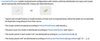
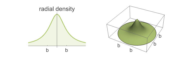
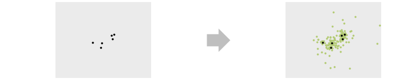
- CauchyPointProcessは,中心が空間内で一様に分布し,クラスタ点が裾が重い動径分布に従って等方的に分布するクラスタ点配置をモデル化する.
- 主に林業等で,例えば種子がその発生源から遠く離れて分散することがあるダイオウマツ等の樹木の位置をモデル化するために使われる.
- クラスタの中心は,密度が μ のPoissonPointProcessに従って分布する.
- クラスタの点の数は,平均が λ のPoissonDistributionに従って分布する.
における各クラスタのクラスタ点はCauchyDistribution[0,b]に従って分布する.
におけるクラスタ点は,クラスタの中心を中心とするMultivariateTDistribution[DiagonalMatrix[{b2,b2,…}],1]に従って分布する.- CauchyPointProcessでは, μ,λ,b は任意の正の実数でよく,d は任意の正の整数でよい.
- PointProcessEstimatorについてCauchyPointProcessを推定するために以下の設定を使うことができる.
-
"FindClusters" FindClusters関数を使う "MethodOfMoments" 均一性尺度を使ってパラメータを推定する - CauchyPointProcessは,RipleyK,PointCountDistribution,RandomPointConfiguration等の関数と一緒に使うことができる.
例題
すべて開く すべて閉じる例 (3)
pts = RandomPointConfiguration[CauchyPointProcess[10, 20, .01, 2], Disk[]]Show[RegionPlot[pts["ObservationRegion"]], ListPlot[pts]]pts = RandomPointConfiguration[CauchyPointProcess[30, 20, .01, 3], Ball[]]Show[RegionPlot3D[pts["ObservationRegion"], PlotStyle -> Opacity[.2], Boxed -> False], ListPointPlot3D[pts]]proc = CauchyPointProcess[.006, .3, .1, 2];pts = RandomPointConfiguration[proc, Entity["Country", "Poland"]]GeoListPlot[pts]スコープ (3)
ℛ = ImplicitRegion[x ^ 2 - 2y ^ 2 <= 1, {{x, -3, 3}, {y, -4, 4}}];{RegionQ[ℛ], RegionEmbeddingDimension[ℛ] == RegionDimension[ℛ]}pts = RandomPointConfiguration[CauchyPointProcess[4, 15, 0.05, 2], ℛ]Show[RegionPlot[pts["ObservationRegion"]], ListPlot[pts]]proc = CauchyPointProcess[20, 30, 1, 2];
points = RandomPointConfiguration[proc, Rectangle[]];PointValuePlot[points]"FindClusters"法を使って点過程モデルを推定する:
est = EstimatedPointProcess[points, CauchyPointProcess[a, b, c, d], PointProcessEstimator -> "FindClusters"]DiscretePlot[{RipleyK[proc, r], RipleyK[est, r]}, {r, 0.1, .5, .005}, PlotLegends -> {"original process", "estimated model"}]pcf = PairCorrelationG[CauchyPointProcess[μ, λ, b, 3], r]Plot[pcf /. {μ -> 3, λ -> 2, b -> 1}, {r, 0, 3}]特性と関係 (6)
PointCountDistributionは既知である:
proc = CauchyPointProcess[4, 15, .1, 2];dist = PointCountDistribution[proc, Disk[]]{Mean[dist], Variance[dist]}DiscretePlot[PDF[dist, x], {x, 50, 400, 5}]sample = RandomVariate[dist, 10 ^ 4];Histogram[sample, 30, "PDF"]2Dにおけるコーシー点過程についてのRipleyの
関数とBesagの
関数:
proc = CauchyPointProcess[μ, λ, b, 2];f1 = RipleyK[proc, r]f2 = BesagL[proc, r]Block[{μ = 20, λ = 10, b = .5}, Plot[{f1, f2}, {r, 0, 1}, PlotLegends -> {"Ripley's K", "Besag's L"}]]コーシー点過程のRipleyの
関数はポアソン(Poisson)点過程についてよりも大きい:
cproc = CauchyPointProcess[μ, λ, b, d];RipleyK[cproc][r]pproc = PoissonPointProcess[μ, d];RipleyK[pproc][r]コーシー点過程についてのBesagの
関数はポアソン点過程についてよりも大きい:
cproc = CauchyPointProcess[μ, λ, b, d];BesagL[cproc][r]//Togetherpproc = PoissonPointProcess[μ, d];BesagL[pproc][r]PairCorrelationG[CauchyPointProcess[μ, λ, b, d], r]PairCorrelationG[PoissonPointProcess[μ, d], r]proc = CauchyPointProcess[4, 15, 0.05, 3];DiscretePlot[EmptySpaceF[proc, r], {r, 0.02, .5, 0.01}]テキスト
Wolfram Research (2020), CauchyPointProcess, Wolfram言語関数, https://reference.wolfram.com/language/ref/CauchyPointProcess.html.
CMS
Wolfram Language. 2020. "CauchyPointProcess." Wolfram Language & System Documentation Center. Wolfram Research. https://reference.wolfram.com/language/ref/CauchyPointProcess.html.
APA
Wolfram Language. (2020). CauchyPointProcess. Wolfram Language & System Documentation Center. Retrieved from https://reference.wolfram.com/language/ref/CauchyPointProcess.html
BibTeX
@misc{reference.wolfram_2026_cauchypointprocess, author="Wolfram Research", title="{CauchyPointProcess}", year="2020", howpublished="\url{https://reference.wolfram.com/language/ref/CauchyPointProcess.html}", note=[Accessed: 19-August-2026]}
BibLaTeX
@online{reference.wolfram_2026_cauchypointprocess, organization={Wolfram Research}, title={CauchyPointProcess}, year={2020}, url={https://reference.wolfram.com/language/ref/CauchyPointProcess.html}, note=[Accessed: 19-August-2026]}