CauchyPointProcess[μ,λ,b,d]
表示
中的一个柯西聚点过程,其密度为 μ,聚类平均值为 λ,缩放参数为 b.
CauchyPointProcess
CauchyPointProcess[μ,λ,b,d]
表示
中的一个柯西聚点过程,其密度为 μ,聚类平均值为 λ,缩放参数为 b.
更多信息
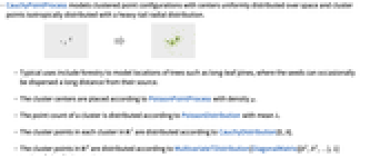
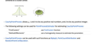
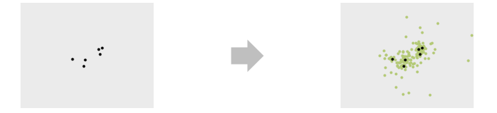
- CauchyPointProcess 模拟聚类点布局,其中心均匀地分布在空间上,聚类点以重尾径向分布方式各向同性地排布在空间中.
-
- 一般用途包括,林业学中为各类树(如长叶松)的位置进行建模,有些种子有的时候可以传播到离其源头很远的地方.
- 聚类中心根据密度为 μ 的 PoissonPointProcess 进行放置.
- 聚类的点数根据平均值为 λ 的 PoissonDistribution 进行分布.
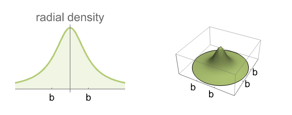
中每个聚类的聚点都根据 CauchyDistribution[0,b] 进行分布.
中的聚点根据聚集在一个聚类中心的 MultivariateTDistribution[DiagonalMatrix[{b2,b2,…}],1] 进行分布.-
- CauchyPointProcess 允许 μ、λ 和 b 为正实数,且 d 为任意正整数.
- PointProcessEstimator 可使用下列设置来计算 CauchyPointProcess:
-
"FindClusters" 使用 FindClusters 函数 "MethodOfMoments" 使用均质性方法计算参数 - CauchyPointProcess 可与诸如 RipleyK、PointCountDistribution 和 RandomPointConfiguration 的函数一起使用.
范例
打开所有单元 关闭所有单元基本范例 (3)
pts = RandomPointConfiguration[CauchyPointProcess[10, 20, .01, 2], Disk[]]Show[RegionPlot[pts["ObservationRegion"]], ListPlot[pts]]pts = RandomPointConfiguration[CauchyPointProcess[30, 20, .01, 3], Ball[]]Show[RegionPlot3D[pts["ObservationRegion"], PlotStyle -> Opacity[.2], Boxed -> False], ListPointPlot3D[pts]]proc = CauchyPointProcess[.006, .3, .1, 2];pts = RandomPointConfiguration[proc, Entity["Country", "Poland"]]GeoListPlot[pts]范围 (3)
ℛ = ImplicitRegion[x ^ 2 - 2y ^ 2 <= 1, {{x, -3, 3}, {y, -4, 4}}];{RegionQ[ℛ], RegionEmbeddingDimension[ℛ] == RegionDimension[ℛ]}pts = RandomPointConfiguration[CauchyPointProcess[4, 15, 0.05, 2], ℛ]Show[RegionPlot[pts["ObservationRegion"]], ListPlot[pts]]proc = CauchyPointProcess[20, 30, 1, 2];
points = RandomPointConfiguration[proc, Rectangle[]];PointValuePlot[points]est = EstimatedPointProcess[points, CauchyPointProcess[a, b, c, d], PointProcessEstimator -> "FindClusters"]比较原始过程和计算出的模型之间的 Ripley
作为度量标准:
DiscretePlot[{RipleyK[proc, r], RipleyK[est, r]}, {r, 0.1, .5, .005}, PlotLegends -> {"original process", "estimated model"}]pcf = PairCorrelationG[CauchyPointProcess[μ, λ, b, 3], r]Plot[pcf /. {μ -> 3, λ -> 2, b -> 1}, {r, 0, 3}]属性和关系 (6)
proc = CauchyPointProcess[4, 15, .1, 2];dist = PointCountDistribution[proc, Disk[]]{Mean[dist], Variance[dist]}DiscretePlot[PDF[dist, x], {x, 50, 400, 5}]sample = RandomVariate[dist, 10 ^ 4];Histogram[sample, 30, "PDF"]二维空间中柯西点过程的 Ripley's
和 Besag's
:
proc = CauchyPointProcess[μ, λ, b, 2];f1 = RipleyK[proc, r]f2 = BesagL[proc, r]Block[{μ = 20, λ = 10, b = .5}, Plot[{f1, f2}, {r, 0, 1}, PlotLegends -> {"Ripley's K", "Besag's L"}]]cproc = CauchyPointProcess[μ, λ, b, d];RipleyK[cproc][r]pproc = PoissonPointProcess[μ, d];RipleyK[pproc][r]cproc = CauchyPointProcess[μ, λ, b, d];BesagL[cproc][r]//Togetherpproc = PoissonPointProcess[μ, d];BesagL[pproc][r]PairCorrelationG[CauchyPointProcess[μ, λ, b, d], r]PairCorrelationG[PoissonPointProcess[μ, d], r]proc = CauchyPointProcess[4, 15, 0.05, 3];DiscretePlot[EmptySpaceF[proc, r], {r, 0.02, .5, 0.01}]文本
Wolfram Research (2020),CauchyPointProcess,Wolfram 语言函数,https://reference.wolfram.com/language/ref/CauchyPointProcess.html.
CMS
Wolfram 语言. 2020. "CauchyPointProcess." Wolfram 语言与系统参考资料中心. Wolfram Research. https://reference.wolfram.com/language/ref/CauchyPointProcess.html.
APA
Wolfram 语言. (2020). CauchyPointProcess. Wolfram 语言与系统参考资料中心. 追溯自 https://reference.wolfram.com/language/ref/CauchyPointProcess.html 年
BibTeX
@misc{reference.wolfram_2026_cauchypointprocess, author="Wolfram Research", title="{CauchyPointProcess}", year="2020", howpublished="\url{https://reference.wolfram.com/language/ref/CauchyPointProcess.html}", note=[Accessed: 09-August-2026]}
BibLaTeX
@online{reference.wolfram_2026_cauchypointprocess, organization={Wolfram Research}, title={CauchyPointProcess}, year={2020}, url={https://reference.wolfram.com/language/ref/CauchyPointProcess.html}, note=[Accessed: 09-August-2026]}