

Circle
Details
- Circle with its different parameter settings is also known as arc, circular arc, semicircle, and ellipse.
- Circle can be used as a geometric region and a graphics primitive.
- Circle[] is equivalent to Circle[{0,0}]. »
- Circle represents the curve
 .
. - Angles are measured in radians counterclockwise from the positive x direction.
- Circle can be used in Graphics.
- In graphics, the point {x,y} and radii r and {rx,ry} can be Scaled, Offset, ImageScaled, and Dynamic expressions.
- Graphics rendering is affected by directives such as Thickness, Dashing, and color.
- Circle can be used with symbolic points and quantities in GeometricScene.
Background & Context
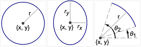
- Circle is a graphics and geometry primitive that represents a circle, ellipse, or circular/elliptical arc in the plane. In particular, Circle[{x,y},r] represents the circle of radius r in
 centered at {x,y}, Circle[{x,y},{rx,ry}] represents the axis-aligned filled ellipse in
  with center {x,y} and semiaxis lengths rx and ry, and Circle[{x,y},…,{θ1,θ2}] represents the (potentially elliptical) arc centered at {x,y} ranging between angles θ1 and θ2 measured in radians counterclockwise from the positive
  axis. The shorthand form Circle[{x,y}] is equivalent to Circle[{x,y},1], while Circle[] autoevaluates to Circle[{0,0},1].
 - Circle objects can be formatted by placing them inside a Graphics expression. Note that while abstract circles have dimension 1 and zero thickness, for convenience, formatted Circle objects are rendered by default with finite thickness. The appearance of Circle objects in graphics can be modified by specifying thickness directives such as Thickness, AbsoluteThickness, Thick and Thin; dashing directives such as Dashing, AbsoluteDashing, Dashed, Dotted and DotDashed; color directives such as Red; the transparency directive Opacity; and the style option Antialiasing.
- Circle may also serve as a region specification over which a computation should be performed. For example, Integrate[1,{x, y}∈Circle[{0,0},r]] and ArcLength[Circle[{x,y},r]] both return the perimeter
 .
. - CirclePoints may be used to give the positions of equally spaced points around a circle.
- Circle is related to a number of other symbols. Circle represents the boundary of a disk, as can be computed using RegionBoundary[Disk[{x,y},r]]. Cylinder and Sphere may be thought of as higher-dimensional analogs of circles. Circle[{x,y},r] may be alternately represented using Sphere[{x,y},r], ImplicitRegion[(x-u)2+(y-v)2r2,{u,v}] or ParametricRegion[{x+r Cos[t],y+r Sin[t]},{t,0,2π}]. Precomputed properties of the circle and its variants in standard position are available using PlaneCurveData["entity","property"] or EntityValue[Entity["PlaneCurve","entity"],"property"], where "entity" is one of "Circle", "CircularArc", "Ellipse", "Semicircle", etc.
Examples
open all close allBasic Examples (5)
Graphics[Circle[]]Graphics[Circle[{0, 0}, 1, {Pi / 6, 3Pi / 4}]]Graphics[Circle[{0, 0}, {3, 4}]]{Graphics[{Red, Circle[]}], Graphics[{Thick, Circle[]}], Graphics[{Dashed, Circle[]}], Graphics[{Red, Thick, Dashed, Circle[]}]}ArcLength of a circle:
ArcLength[Circle[]]ArcLength[Circle[{0, 0}, 1, {Pi / 6, 3Pi / 4}]]Scope (23)
Graphics (13)
Specification (6)
Graphics[{Circle[{0, 0}, 1], Circle[{0, 0}, 3], Circle[{0, 0}, 5]}]Graphics[{Circle[{0, 0}, 1], Circle[{1, 1}, 1], Circle[{2, 2}, 1]}]Graphics[Circle[{0, 0}, 1, {0, 4Pi / 3}]]Graphics[Circle[{0, 0}, 1, {4Pi / 3, 2Pi}]]Graphics[Circle[{0, 0}, {3, 2}]]Graphics[Circle[{0, 0}, {3, 2}, {0, 4Pi / 3}]]Short form for a unit circle at the origin:
Graphics[Circle[], Axes -> True]Styling (3)
Circles with different thicknesses:
Table[Graphics[{Thickness[i], Circle[]}], {i, {Tiny, Small, Medium, Large}}]Table[Graphics[{Thickness[i], Circle[]}], {i, {.05, .1, .2}}]Thickness in printer's points:
Table[Graphics[{AbsoluteThickness[i], Circle[]}], {i, {1, 5, 10}}]{Graphics[{Dashed, Circle[]}], Graphics[{Dotted, Circle[]}], Graphics[{DotDashed, Circle[]}]}Table[Graphics[{c, Circle[]}], {c, {Red, Green, Blue, Yellow}}]Coordinates (4)
Using Scaled coordinates and radii:
Graphics[Circle[Scaled[{.2, .2}], .2], Frame -> True]Graphics[Circle[{0, 0}, Scaled[.25]], Frame -> True]Graphics[Circle[{0, 0}, Scaled[{.5, .25}]], Frame -> True]Use ImageScaled coordinates and radii:
Graphics[Circle[ImageScaled[{.2, .2}], .2], Frame -> True]Graphics[Circle[{0, 0}, ImageScaled[{.5, .25}]], Frame -> True]Use Offset coordinates:
Graphics[Circle[Offset[{10, 10}, {0, 0}], .5], Frame -> True]Use Offset to specify the radii in printer's points:
Graphics[Circle[{0, 0}, Offset[{10, 40}]], Frame -> True]Regions (10)
RegionEmbeddingDimension[Circle[{Subscript[c, 1], Subscript[c, 2]}, r]]RegionDimension[Circle[{Subscript[c, 1], Subscript[c, 2]}, r]]{RegionMember[Circle[], {0, 1}], RegionMember[Circle[], {0, 0}]}Get conditions for point membership:
RegionMember[Circle[{Subscript[c, 1], Subscript[c, 2]}, {Subscript[r, 1], Subscript[r, 2]}], {x, y}]ℛ = Circle[];{ArcLength[ℛ], RegionMeasure[ℛ]}c = RegionCentroid[ℛ]Graphics[{{Gray, ℛ}, {Red, Point[c]}}]ℛ = Circle[];{RegionDistance[ℛ, {1, 1}], RegionDistance[ℛ, {1, 0}]}The distance to the nearest point for the unit circle:
{Plot3D[Evaluate@RegionDistance[ℛ, {x, y}], {x, -2, 2}, {y, -2, 2}, MeshFunctions -> {#3&}, Mesh -> 5, Exclusions -> Norm[{x, y}] == 1], ContourPlot[Evaluate@RegionDistance[ℛ, {x, y}], {x, -3, 3}, {y, -3, 3}, Contours -> {{0.5, Red}, {1, Green}, {1.5, Blue}}]}ℛ = Circle[];{SignedRegionDistance[ℛ, {1, 1}], SignedRegionDistance[ℛ, {1, 0}]}Signed distance to the unit circle:
Plot3D[SignedRegionDistance[ℛ, {x, y}], {x, -2, 2}, {y, -2, 2}, Exclusions -> Norm[{x, y}] == 1, Mesh -> None]ℛ = Circle[{0, 0}, {3, 2}];{RegionNearest[ℛ, {0, 3}], RegionNearest[ℛ, {3, 0}]}pts = Join[Table[4{Cos[k 2 π / 10], Sin[k 2π / 10]}, {k, 0., 9}],
Table[{k, 0}, {k, -3., 3, 0.6}]];
nst = RegionNearest[ℛ, #]& /@ pts;Legended[Graphics[{ℛ, {Thin, StandardGray, Line[Transpose[{pts, nst}]]}, {StandardRed, Point[pts]}, {StandardCyan, Point[nst]}}], PointLegend[{StandardRed, StandardCyan}, {"start", "nearest"}]]ℛ = Circle[];BoundedRegionQ[ℛ]rr = RegionBounds[ℛ]Graphics[{{EdgeForm[Directive[Dashed, Red]], Opacity[0.1], Yellow, Rectangle@@Transpose[rr]}, ℛ}]Integrate over a circle:
ℛ = Circle[{Subscript[c, 1], Subscript[c, 2]}, r];Integrate[x y, {x, y}∈ℛ]ℛ = Circle[{1, 2}, 3];Minimize[{x y - x, {x, y}∈ℛ}, {x, y}]//Simplifyℛ = Circle[{1, 2}, 3];Solve[y == 2x + 1 && {x, y}∈Circle[], {x, y}]Graphics[{{StandardBlue, Circle[]}, {Gray, InfiniteLine[{0, 1}, {1, 2}]}, {Red, PointSize[Medium], Point[{x, y} /. %]}}, Frame -> True]Applications (8)
The square packing of circles:
Graphics[Table[Circle[{i, j}, 1 / 2], {i, 7}, {j, 5}]]The hexagonal packing of circles:
Graphics[Table[Circle[{i + ((-1) ^ j + 1) / 4, Sqrt[3] / 2j}, 1 / 2], {i, 7}, {j, 5}]]Simulation of elliptical gears:
Animate[Module[{a = 4, b = 3, f, r}, f = Sqrt[a ^ 2 - b ^ 2];r = b ^ 2 / (a + f Cos[θ]);Graphics[{Point[{{0, 0}, {2a, 0}}], Rotate[Circle[{-f, 0}, {a, b}], θ, {0, 0}], Translate[Rotate[Circle[{-f, 0}, {a, b}], -ArcTan[ 2 f + r Cos[θ], r Sin[θ]], {0, 0}], {2a, 0}]}, PlotRange -> {{-2a, 4a}, {-2a, 2a}}, ImageSize -> 250]], {θ, 0, 2Pi}, AnimationRunning -> False]Find the intersections of a Line and a Circle:
Subscript[ℛ, 1] = Line[{{-2, -1}, {5, 6}}];
Subscript[ℛ, 2] = Circle[{1, 2}, 3];pts = Solve[{x, y}∈Subscript[ℛ, 1] && {x, y}∈Subscript[ℛ, 2], {x, y}]Graphics[{Subscript[ℛ, 1], Subscript[ℛ, 2], {Red, PointSize[Medium], Point[{x, y} /. pts]}}]Find the intersections of two circles:
Subscript[ℛ, 1] = Circle[{-1, 0}, 3];
Subscript[ℛ, 2] = Circle[{1, 0}, 3];pts = Solve[{x, y}∈Subscript[ℛ, 1] && {x, y}∈Subscript[ℛ, 2], {x, y}]Graphics[{Subscript[ℛ, 1], Subscript[ℛ, 2], {Red, PointSize[Medium], Point[{x, y} /. pts]}}]Illustrate a function's radius of curvature:
y[x_] := Sin[x ^ 2];
r[x_] := ((1 + y'[x] ^ 2) ^ (3 / 2)) / y''[x];
c[x_] := Circle[{x, y[x]} + r[x]Normalize[{-y'[x], 1}], Abs[r[x]]];Show[{Plot[y[x], {x, -2, 2}], Graphics[{c[-1.2], c[0], c[1.4], Red, PointSize[Medium], Point[{-1.2, y[-1.2]}], Point[{0, y[0]}], Point[{1.4, y[1.4]}]}]}, AspectRatio -> Automatic]A circumcircle is a circle in the plane defined by three noncollinear points:
pts = {{0, 1}, {-2 / 3, -1 / 3}, {3 / 4, 0}};
circ = Circumsphere[pts];Graphics[{circ, StandardBlue, Triangle[pts]}]The radius and circumcenter can be extracted from the Circumsphere:
{c, r} = {First[circ], Last[circ]}Graphics[{circ, StandardBlue, Triangle[pts], Red, Point[c], Dashed, Line[{c, c + r * Normalize[{1, 1}]}]}]The defining property of a DelaunayMesh is that no input point is contained in the circumcircle of any Triangle in the mesh:
SeedRandom[1234];
ℛ = DelaunayMesh[RandomReal[1, {8, 2}]];
circles = Circumsphere@@@Normal@GraphicsComplex[MeshCoordinates[ℛ], MeshCells[ℛ, 2]];Show[HighlightMesh[ℛ, Style[{0, All}, Directive[Red, PointSize[Medium]]]], Graphics[{Gray, circles}], PlotRange -> {{0, 1}, {0, 1}}]Given electric charge density along a circular wire, use Integrate to find the total charge:
charge[x_, y_] := x ^ 4 + y ^ 2;ParametricPlot3D[{Cos[θ], Sin[θ], charge[Cos[θ], Sin[θ]]z}, {θ, 0, 2π}, {z, 0, 1}, Mesh -> None]Integrate[charge[x, y], {x, y}∈Circle[]]Properties & Relations (10)
Use Rotate to get all possible ellipses:
Graphics[Rotate[Circle[{0, 0}, {4, 2}], Pi / 6], Axes -> True]To create a filled circle, use Disk:
Graphics[{Pink, Disk[]}]The 3D generalization is Sphere:
Graphics3D[Sphere[]]An implicit specification of a circle can be generated by ContourPlot:
ContourPlot[x ^ 2 + y ^ 2 == 1, {x, -1, 1}, {y, -1, 1}]A parametric specification of a circle can be generated by ParametricPlot:
ParametricPlot[{Cos[θ], Sin[θ]}, {θ, 0, 2π}]Sphere can represent any Circle:
Subscript[ℛ, 1] = Sphere[{x, y}, r];
Subscript[ℛ, 2] = Circle[{x, y}, r];RegionEqual[Subscript[ℛ, 1], Subscript[ℛ, 2]]Circumsphere can represent any Circle:
Subscript[ℛ, 1] = Circumsphere[{{1, 0}, {0, 1}, {-1, 0}}];
Subscript[ℛ, 2] = Circle[{0, 0}, 1];RegionEqual[Subscript[ℛ, 1], Subscript[ℛ, 2]]ParametricRegion can represent any Circle:
Subscript[ℛ, 1] = ParametricRegion[{{1 + 3Cos[t], 2 + 4 Sin[t]}, 0 ≤ t ≤ 2π}, {t}];
Subscript[ℛ, 2] = Circle[{1, 2}, {3, 4}];RegionEqual[Subscript[ℛ, 1], Subscript[ℛ, 2]]ImplicitRegion can represent any Circle:
Subscript[ℛ, 1] = ImplicitRegion[x^2 + y^2 == 1, {x, y}];
Subscript[ℛ, 2] = Circle[{0, 0}, 1];RegionEqual[Subscript[ℛ, 1], Subscript[ℛ, 2]]Circle is a norm circle for the Euclidean norm:
ℛ = Circle[{0, 0}, 1];Reduce[{x, y}∈ℛ⧦Norm[{x, y}] == 1, {x, y}, Reals]Possible Issues (2)
Using Scaled radii will depend on the PlotRange:
Table[Graphics[Circle[{0, 0}, Scaled[.25]], PlotRange -> {{-n, n}, {-1, 1}}, Frame -> True, FrameTicks -> {{{-1, 1}, None}, {{-n, n}, None}}], {n, {1, 2, 3}}]Using ImageScaled sizes will depend on the ImageSize and AspectRatio:
Table[Graphics[Circle[ImageScaled[{.5, .5}], ImageScaled[{.25, .25}]], Frame -> True, FrameTicks -> {{{-1, 1}, None}, {{-1, 1}, None}}, ImageSize -> n], {n, {50, 70, 100}}]Table[Graphics[Circle[ImageScaled[{.5, .5}], ImageScaled[{.25, .25}]], Frame -> True, FrameTicks -> {{{-1, 1}, None}, {{-1, 1}, None}}, ImageSize -> 100, AspectRatio -> n], {n, {1, 1 / 2, 1 / 3}}]Neat Examples (4)
Graphics[Table[{Hue[RandomReal[]], Circle[RandomReal[4, {2}], RandomReal[1]]}, {40}]]Graphics[{Thick, Orange, Circle[], Table[Circle[{Cos[2 Pi i / 6], Sin[2Pi i / 6]}, 1], {i, 6}]}]Graphics[Table[{Hue[t / 20], Circle[{Cos[2Pi t / 20], Sin[2Pi t / 20]}, 1]}, {t, 20}]]Animate[Graphics[{Thick, Circle[{0, 0}, 2, {0, Pi}], Circle[{0, 0}, 2, {Pi, 2Pi}], Circle[{-1, 0}, 1, {Pi, 2Pi}], Circle[{1, 0}, 1, {0, Pi}]}, PlotRange -> 2.1, ImageSize -> 150] /. Circle[x__] :> Rotate[Circle[x], d Degree, {0, 0}], {d, 0, 360}, AnimationRunning -> False]Related Links
Text
Wolfram Research (1991), Circle, Wolfram Language function, https://reference.wolfram.com/language/ref/Circle.html (updated 2014).
CMS
Wolfram Language. 1991. "Circle." Wolfram Language & System Documentation Center. Wolfram Research. Last Modified 2014. https://reference.wolfram.com/language/ref/Circle.html.
APA
Wolfram Language. (1991). Circle. Wolfram Language & System Documentation Center. Retrieved from https://reference.wolfram.com/language/ref/Circle.html