CoshIntegral

CoshIntegral[z]

双曲線余弦積分を与える．

詳細

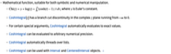
記号操作・数値操作の両方に適した数学関数である．
$TemplateBox[{z}, CoshIntegral]=gamma+log(z)+int_0^z(cosh(t)-1)/tdt$ ，ただしはオイラーの定数である．
CoshIntegral[z]は，複素 z 平面上，-∞〜0の範囲で不連続な分枝切断線を持つ．
特別な引数の場合，CoshIntegralは，自動的に厳密値を計算する．
CoshIntegralは任意の数値精度で評価できる．
CoshIntegralは，自動的にリストに縫い込まれる．
CoshIntegralはIntervalオブジェクトおよびCenteredIntervalオブジェクトに使うことができる． »

例題

すべて開くすべて閉じる

例 (6)

数値的に評価する：

Wolfram Language code: CoshIntegral[2.8]

実数の部分集合上でプロットする：

Wolfram Language code: Plot[CoshIntegral[x], {x, 0, 5}]

複素数の部分集合上でプロットする：

Wolfram Language code: ComplexPlot3D[CoshIntegral[z], {z, -2 - 2I, 2 + 2I}, PlotLegends -> Automatic]

原点における級数展開：

Wolfram Language code: Series[CoshIntegral[x], {x, 0, 10}]

Infinityにおける漸近展開：

Wolfram Language code: Series[CoshIntegral[x], {x, ∞, 3}]//Normal

特異点における漸近展開：

Wolfram Language code: Series[CoshIntegral[x], {x, -1, 3}, Assumptions -> x > 0]//Normal

スコープ (38)

数値評価 (6)

高精度で評価する：

Wolfram Language code: N[CoshIntegral[2], 50]

出力の精度は入力の精度に従う：

Wolfram Language code: CoshIntegral[2.000000000000000000000000000000000000]

複素引数について評価する：

Wolfram Language code: CoshIntegral[3.5 + I]

CoshIntegralを高精度で効率よく評価する：

Wolfram Language code: CoshIntegral[2`500]//Timing

Wolfram Language code: CoshIntegral[2`10000];//Timing

CoshIntegralは要素単位でリストに縫い込まれる：

Wolfram Language code: CoshIntegral[{1.2, 1.5, 1.8}]

IntervalオブジェクトとCenteredIntervalオブジェクトを使って最悪の場合に保証される区間を計算する：

Wolfram Language code: CoshIntegral[Interval[{1.9, 2.1}]]

Wolfram Language code: CoshIntegral[CenteredInterval[2, 1 / 100]]

Aroundを使って平均的なケースの統計区間を計算することもできる：

Wolfram Language code: CoshIntegral[Around[2, 0.01]]

配列の要素ごとの値を計算する：

Wolfram Language code: CoshIntegral[{{.1, 0}, {0, .1 }}]

MatrixFunctionを使って行列のCoshIntegral関数を計算することもできる：

Wolfram Language code: MatrixFunction[CoshIntegral, {{.1, 0}, {0, .1 }}]

特定の値 (3)

原点における値：

Wolfram Language code: CoshIntegral[0]

無限大における値：

Wolfram Language code: CoshIntegral[{Infinity, -I Infinity, I Infinity}]

Wolfram Language code: CoshIntegral[ComplexInfinity]

CoshIntegralの零点を求める：

Wolfram Language code: xzero = Solve[CoshIntegral[x] == 0 && 0 < x < 1.0, x][[1, 1, 2]]//Quiet

Wolfram Language code: Plot[CoshIntegral[x], {x, 0, 2}, Epilog -> Style[Point[{xzero, CoshIntegral[xzero]}], PointSize[Large], Red]]

可視化 (2)

CoshIntegral関数をプロットする：

Wolfram Language code: Plot[CoshIntegral[x], {x, 0, 7}]

の実部をプロットする：

Wolfram Language code: ComplexContourPlot[Re[CoshIntegral[z]], {z, -4 - 8 I, 4 + 8 I}, Contours -> 24]

の虚部をプロットする：

Wolfram Language code: ComplexContourPlot[Im[CoshIntegral[z]], {z, -4 - 8 I, 4 + 8 I}, Contours -> 24]

関数の特性 (9)

CoshIntegralはすべての正の実数値について定義される：

Wolfram Language code: FunctionDomain[CoshIntegral[x], x]

複素領域：

Wolfram Language code: FunctionDomain[CoshIntegral[z], z, Complexes]

CoshIntegralはすべての実数値を取る：

Wolfram Language code: FunctionRange[CoshIntegral[x], x, y]

CoshIntegralは解析関数ではない：

Wolfram Language code: FunctionAnalytic[CoshIntegral[x], x]

有理型でもない：

Wolfram Language code: FunctionMeromorphic[CoshIntegral[x], x]

CoshIntegralは実領域上で増加する：

Wolfram Language code: FunctionMonotonicity[{CoshIntegral[x], x > 0}, x, StrictInequalities -> True]

CoshIntegralは単射である：

Wolfram Language code: FunctionInjective[CoshIntegral[x], x]

Wolfram Language code: Plot[{CoshIntegral[x], 2}, {x, 0, 5}]

CoshIntegralは全射である：

Wolfram Language code: FunctionSurjective[CoshIntegral[x], x]

Wolfram Language code: Plot[{CoshIntegral[x], 200}, {x, 0, 10}]

CoshIntegralは非負でも非正でもない：

Wolfram Language code: FunctionSign[{CoshIntegral[x], x > 0}, x]

(-∞,0]に特異点と不連続点の両方を持つ：

Wolfram Language code: FunctionSingularities[CoshIntegral[x], x]

Wolfram Language code: FunctionDiscontinuities[CoshIntegral[x], x]

CoshIntegralは凸でも凹でもない：

Wolfram Language code: FunctionConvexity[{CoshIntegral[x], x > 0}, x]

微分 (3)

一次導関数：

Wolfram Language code: D[CoshIntegral[x], x]

高次導関数：

Wolfram Language code: Table[D[CoshIntegral[x], {x, n}], {n, 1, 4}]//Simplify

Wolfram Language code:

Plot[Evaluate[%], {x, -3, 3}, PlotLegends -> {"First Derivative", "Second Derivative", "Third Derivative", "Fourth Derivative"}]

次導関数の式：

Wolfram Language code: D[CoshIntegral[x], {x, n}]

積分 (3)

CoshIntegralの不定積分：

Wolfram Language code: Integrate[CoshIntegral[x], x]

定積分：

Wolfram Language code: Integrate[CoshIntegral[x], {x, -1, 0}]

その他の積分例：

Wolfram Language code: Integrate[CoshIntegral[z^a], z]

Wolfram Language code: Integrate[CoshIntegral[x]Exp[-a x], {x, 0, Infinity}, Assumptions -> a > 1]

級数展開 (3)

CoshIntegralの級数展開：

Wolfram Language code: Series[CoshIntegral[x], {x, 0, 5}]

の周りのCoshIntegralの最初の3つの近似をプロットする：

Wolfram Language code:

terms = Normal@Table[Series[CoshIntegral[x], {x, 0, m}], {m, 1, 5, 2}];
Plot[{CoshIntegral[x], terms}, {x, 0, 4}]

無限大における漸近的な級数展開を求める：

Wolfram Language code: Series[CoshIntegral[x], {x, Infinity, 3}]

CoshIntegralはベキ級数に適用できる：

Wolfram Language code: CoshIntegral[1 + x + (x^2/2) + (x^3/9) + O[x]^4]

積分変換 (2)

LaplaceTransformを使ってラプラス(Laplace)変換を計算する：

Wolfram Language code: LaplaceTransform[CoshIntegral[t], t, s, Assumptions -> Re[s] > 1]

HankelTransform：

Wolfram Language code: HankelTransform[CoshIntegral[r], r, s ]//FullSimplify

関数の恒等式と簡約 (3)

CoshIntegralの主定義：

Wolfram Language code: Integrate[(Cosh[t] - 1/t), {t, 0, z}] + Log[z] + EulerGamma

引数の簡約：

Wolfram Language code: CoshIntegral[-z] == CoshIntegral[z] + Log[-z] - Log[z]//FullSimplify

Wolfram Language code: CoshIntegral[Sqrt[z^2]]//FunctionExpand

式を簡約してCoshIntegralにする：

Wolfram Language code: -(1/2)(Gamma[0, -z] + Gamma[0, z] + Log[-z] - Log[z])//FullSimplify

関数表現 (4)

CosIntegralとLogによる表現：

Wolfram Language code: CosIntegral[I z] - Log[I z] + Log[z]//FullSimplify

CoshIntegralはMeijerGによって表すことができる：

Wolfram Language code: MeijerGReduce[CoshIntegral[x], x]

Wolfram Language code: Activate[%]//FullSimplify

CoshIntegralはDifferentialRootとして表すことができる：

Wolfram Language code: DifferentialRootReduce[CoshIntegral[x], x]

TraditionalFormによる表示：

Wolfram Language code: CoshIntegral[x]//TraditionalForm

アプリケーション (3)

複素平面上で虚部をプロットする：

Wolfram Language code: Plot3D[Im[CoshIntegral[x + I y]], {x, -3, 3}, {y, -10, 10}]

微分方程式を解く：

Wolfram Language code: DSolve[y'[x] - y[x] - CoshIntegral[x] == 0, y[x], x]

DSolveValueを使って不定積分を求める：

Wolfram Language code: DSolveValue[y'[x] - CoshIntegral[x] == 0, y[x], x]

Integrateが与える答と比較する：

Wolfram Language code: Integrate[CoshIntegral[x], x, GeneratedParameters -> C]

特性と関係 (3)

FullSimplifyを使って双曲線余弦積分を含む式を簡約する：

Wolfram Language code: FullSimplify[CoshIntegral[z] - (z^2/4)HypergeometricPFQ[{1, 1}, {2, 2, (3/2)}, (z^2/4)]]

FunctionExpandを使って他の関数を通してCoshIntegralを表現する：

Wolfram Language code: FunctionExpand[CoshIntegral[z] - CoshIntegral[-z]]

近似根を数値的に求める：

Wolfram Language code: FindRoot[CoshIntegral[z] == Pi, {z, 1}]

積分と総和からCoshIntegralを求める：

Wolfram Language code: Integrate[(Cosh[t] - 1/t), {t, 0, z}]

Wolfram Language code: Underoverscript[∑, k = 1, ∞]( z^2 k/k (2 k)!)

考えられる問題 (2)

CoshIntegralは中程度の大きさの引数の大きい値を取ることができる：

Wolfram Language code: CoshIntegral[10. ^ 6 ]

$MaxExtraPrecisionの設定値を大きくする必要があるかもしれない：

Wolfram Language code: N[CoshIntegral[I 10 ^ 60 ] - Pi / 2 I, 20]

Wolfram Language code: Block[{$MaxExtraPrecision = 150}, N[CoshIntegral[I 10 ^ 60 ] - Pi / 2 I, 20]]

おもしろい例題 (2)

ネストした積分：

Wolfram Language code: NestList[Integrate[#, x]&, CoshIntegral[ x], 4]

絶対値の対数を複素平面上でプロットする：

Wolfram Language code: ContourPlot[Log[Abs[CoshIntegral[x + I y]]], {x, -10, 10}, {y, -10, 10}]

Top

その他のラーニングリソース

テクニカルサポート

Wolframソリューション

教育のためのWolframソリューション

使い始める

Grow Your Skills

Wolframと繋がる

大人用の教育プログラム

若者のための教育プログラム

読む

CoshIntegral

詳細

例題

例 (6)