CoxModelFit[{e1,…,en}]
事象時間 eiについてのベースラインハザード
のモデルを構築する.
CoxModelFit[{{{ξ11,…,ξ1p},…,{ξn1,…,ξnp}},{e1,…,en}},{f1,…,fm},{x1,…,xp}]

の形式のコックス(Cox)モデルを構築する.ただし,fi は xkに依存するものとする.

CoxModelFit
CoxModelFit[{e1,…,en}]
事象時間 eiについてのベースラインハザード
のモデルを構築する.
CoxModelFit[{{{ξ11,…,ξ1p},…,{ξn1,…,ξnp}},{e1,…,en}},{f1,…,fm},{x1,…,xp}]
の形式のコックス(Cox)モデルを構築する.ただし,fi は xkに依存するものとする.

詳細とオプション

- CoxModelFitは,生存率,信頼性,デュレーションの分析に使われる.これは相対的な生存リスクを数量化し,潜在するベースラインハザードを推定する.
- CoxModelFitはこれが構築する比例ハザードモデルを表す記号CoxModelオブジェクトを返す.モデルの特性と診断は model["property"]で得ることができる.
- 使用可能なモデル特性のリストは model["Properties"]で得ることができる.
- 事象 eiの形式はEventDataで使われた形式に従う.
- CoxModelFitは,ベースラインハザード関数
に比例する条件付きハザード関数
を作成する. - このモデルはセミパラメトリックで,母数
は部分尤度を最大にして求まる.ベースラインハザード
はノンパラメトリックな方法で推定される.
のみを推定する帰無モデルはCoxModelFit[{ξ,e},{},{x1,…,xp}]と等価であるCoxModelFit[e]を用いて指定できる.- 基底関数 fiで指定される定数値はフィットの過程では無視され,ベースラインハザード
の推定に吸収される. - 以下の特性値の表は,モデルのパラメトリック成分
の推定,診断,検定と関連するものである. » - model["property"]で得られるデータとフィットされた関数に関連する特性
-
"BaselineList" 各層のベースライン共変量の水準を含むリスト "BasisFunctions" 基底関数
のリスト"BestFitParameters" 母数推定 
"Data" 共変量入力データ
の行列"EventData" 事象入力データ 
"RelativeRisk" モデル母数の相対的リスク 
"StrataModels" 各層のサブモデルを含むリスト "StrataSummary" 各層の名前と数のペアを含むリスト - 適合度フィットを測る特性
-
"AIC" 赤池情報量基準 "BIC" Schwartz–Bayes情報量基準 "LogLikelihood" モデル対数尤度 "MaxRSquared" 可能な最大
係数"RSquared" 擬似決定係数 
- 残差と影響の尺度タイプ
-
"BetaDifferences" 母数値に対する影響のDFBETAs尺度 "CoxSnellResiduals" Cox–Snell型残差 "DevianceResiduals" スケールされたマルチンゲール(Martingale)残差 "MartingaleResiduals" 時間の経過における事象の超過数の推定 "ScaledBetaDifferences" モデルの標準偏差を使って計算されたDFBETAs "SchoenfeldResiduals" Schoenfeld型残差 "ScoreResiduals" スコア残差 - 母数推定の特性と診断に含まれるもの
-
"CovarianceMatrix" モデル母数の共分散推定 "InformationMatrix" モデル母数の情報行列 "LikelihoodRatioStatistic" フィットされたモデルと帰無モデルの尤度比 "ParameterConfidenceIntervals" 母数推定についての信頼区間 "ParameterStandardErrors" モデル母数の標準誤差 "ParameterTable" フィットされた母数情報の表 "ParameterTableEntries" 母数表の項目 "RelativeRiskConfidenceIntervals" 相対的なリスク推定の信頼区間 "RiskScores" 各観察のリスクスコア "ScoreStatistic" フィットされたモデルと帰無モデルを比較するスコア統計 "TestTable" モデル母数の有意性情報の表 "TestTableEntries" 検定表からの項目 "TestTableEntriesFunction" 検定表関数を使って作られた表からの項目 "TestTableFunction" 指定された帰無仮説のもとでの検定表を作成 "WaldStatistic" フィットされたモデルと帰無モデルを比較するWald統計 - SurvivalModelFitにおけるように,生存確率の推定,生存率の信頼区間,モーメント推定を含むモデル
のノンパラメトリック成分の情報を得ることは可能である. » - CoxModelFitにはSurvivalModelFitで使用可能なすべての特性がある.
に関連する特性はSurvivalModelFitにおけるのと同じように指定される.これに加えて共変量の水準 x0が model["property"][x0]として与えられなければならない.- model[h][x0]の形式 h を指定することで,共変量の水準 x0のハザード比
の異なる関数形式が得られる.次は使用可能な形式である. -
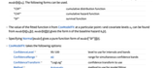
"CDF" 累積分布関数 "CHF" 累積ハザード関数 "SF" 生存関数 - CoxModelFitからの特定の点 t における共変量の水準が x0のフィットされた関数 h の値はmodel[h][x0][t]で得ることができる.model[h][][t]はベースラインハザード h0[t]の形式 h を与える.
- Normal[model]を指定すると model["SF"][][t]の純関数形が得られる.
- CoxModelFitの使用可能なオプション
-
ConfidenceLevel 95/100 区間と帯域に使うレベル ConfidenceRange All 同時信頼帯の範囲 ConfidenceTransform "LogLog" 使用する信頼変換 Method Automatic モデルのフィットに使用するメソッド NominalVariables None カテゴリ的と考えられる変数 StrataVariables None 層的と考えられる変数 WorkingPrecision Automatic 内部計算精度 - ConfidenceLevel->p のとき,確率 p の信頼区間と信頼帯はさまざまな関数形式と母数推定について計算される.
- ConfidenceRange->{tmin,tmax}はフィットされた関数の tminから tmaxまでの確率 p の同時信頼区間と信頼帯を与える.
- ConfidenceTransformの使用可能な設定値には,"Linear","LogLog","ArcSinSqrt", "Log","Logit",あるいは純関数 g がある.
- Method->m という設定はタイを扱う方法を指定する.次は使用可能な設定値である.
-
"Breslow" Breslowの部分尤度を使う "Efron" Efronの部分尤度を使う "Exact" 厳密な周辺尤度を使う - デフォルトで,タイを扱う際には"Breslow"メソッドが使われる.
- 例題のオプションの項目にその他のメソッド設定があるので参照されたい. »
例題
すべて開く すべて閉じる例 (2)
コックス比例ハザードモデルを右打切り事象時間のあるデータにフィットする:
ξ = {2, 0, 0, 1, 1, 1, 3, 0, 0, 1, 1, 0, 0, 0, 0, 1, 1, 0, 0, 0};
e = EventData[Automatic, {{8, 22, 6, 4, 12, 11, 2, 34, 25, 15, 8, 6, 34, 6, 32, 1, 15, 9, 9, 6},
{0, 0, 0, 0, 0, 0, 0, 1, 1, 0, 0, 0, 1, 1, 1, 0, 0, 1, 1, 0}, None}];𝒮 = CoxModelFit[{ξ, e}, x, x]Plot[Evaluate@Table[𝒮["SF"][{x}][t], {x, r = {0, 1, 2, 3}}], {t, 0, 35}, PlotPoints -> 75, Exclusions -> None, PlotLegends -> (Row[{"x = ", #}]& /@ r)]e = EventData[{1, 2, 3, 4}, {0, 0, 1, 0}];𝒮 = CoxModelFit[{{2, 1, 3, 1}, e}, x, x]𝒮["ParameterTable"]𝒮["TestTable"]スコープ (26)
基本的な用法 (8)
ξ = {{67, 1}, {11, 0}, {32, 0}, {50, 1}, {65, 1}, {44, 1}, {20, 1}, {26, 0}, {69, 1}, {50, 1}, {25, 1}, {18, 0}, {63, 1}, {41, 0}, {30, 0}, {32, 1}, {46, 1}, {35, 0}, {33, 0}, {22, 0}};𝒮 = CoxModelFit[{ξ, EventData[Automatic, {{8, 22, 6, 4, 12, 11, 2, 34, 25, 15, 8, 6, 34, 6, 32, 1, 15, 9, 9, 6},
{0, 0, 0, 0, 0, 0, 0, 1, 1, 0, 0, 0, 1, 1, 1, 0, 0, 1, 1, 0}, None}]}, {Subscript[x, 1], Subscript[x, 2]}, {Subscript[x, 1], Subscript[x, 2]}];
と
についての母数推定は5%の水準で両方とも0から有意に隔たっている:
𝒮["ParameterTable"]フィットされたモデルを共変量を含まない帰無モデルと比較する:
𝒮["TestTable"]相対的なリスクと母数推定について95%の信頼区間を形成する:
𝒮["RelativeRiskConfidenceIntervals"]𝒮["ParameterConfidenceIntervals"]ξ = {{67, 1}, {11, 0}, {32, 0}, {50, 1}, {65, 1}, {44, 1}, {20, 1}, {26, 0}, {69, 1}, {50, 1}, {25, 1}, {18, 0}, {63, 1}, {41, 0}, {30, 0}, {32, 1}, {46, 1}, {35, 0}, {33, 0}, {22, 0}};𝒮 = CoxModelFit[{ξ, EventData[Automatic, {{8, 22, 6, 4, 12, 11, 2, 34, 25, 15, 8, 6, 34, 6, 32, 1, 15, 9, 9, 6},
{0, 0, 0, 0, 0, 0, 0, 1, 1, 0, 0, 0, 1, 1, 1, 0, 0, 1, 1, 0}, None}]}, {Subscript[x, 1], Subscript[x, 2]}, {Subscript[x, 1], Subscript[x, 2]}];
が25に固定されているときの,さまざまな水準の
の生存率をベースラインの生存率と比較する:
Plot[Evaluate@{𝒮["SF"][{25, 0}][t], 𝒮["SF"][{25, 1}][t], 𝒮["SF"][][t]}, {t, 0, 35}, Exclusions -> None, PlotPoints -> 100, PlotLegends -> {"SubscriptBox[x, 2] = 0", "SubscriptBox[x, 2] = 1", "baseline"}]
が25に固定されているときの,
の2つの水準の生存時間の中央値を計算する:
𝒮["MedianSurvival"][#]& /@ {{25, 0}, {25, 1}}𝒮["MedianSurvival"][]𝒮["SF"][{30, 0}][20]𝒮["PointwiseBands", "SF"][{30, 0}][20]ξ = {{67, 1}, {11, 0}, {32, 0}, {50, 1}, {65, 1}, {44, 1}, {20, 1}, {26, 0}, {69, 1}, {50, 1}, {25, 1}, {18, 0}, {63, 1}, {41, 0}, {30, 0}, {32, 1}, {46, 1}, {35, 0}, {33, 0}, {22, 0}};𝒮S = CoxModelFit[{ξ, EventData[Automatic, {{8, 22, 6, 4, 12, 11, 2, 34, 25, 15, 8, 6, 34, 6, 32, 1, 15, 9, 9, 6},
{0, 0, 0, 0, 0, 0, 0, 1, 1, 0, 0, 0, 1, 1, 1, 0, 0, 1, 1, 0}, None}]}, {Subscript[x, 1]}, {Subscript[x, 1], Subscript[x, 2]}, StrataVariables -> Subscript[x, 2]];𝒮S["StrataSummary"]水準
と水準
について異なる形式のハザード関数をプロットする:
Table[Plot[𝒮S[i][{60, 1}][t], {t, 0, 20}, PlotLabel -> i, Exclusions -> None], {i, {"SF", "CDF", "CHF"}}]𝒮S["ParameterTable"]ξ = {{67, "Orange"}, {11, "Blue"}, {32, "Blue"}, {50, "Orange"}, {65, "Orange"}, {44, "Orange"}, {20, "Orange"}, {26, "Blue"}, {69, "Orange"}, {50, "Orange"}, {25, "Orange"}, {18, "Blue"}, {63, "Orange"}, {41, "Blue"}, {30, "Blue"}, {32, "Orange"}, {46, "Orange"}, {35, "Blue"}, {33, "Blue"}, {22, "Blue"}};𝒮 = CoxModelFit[{ξ, EventData[Automatic, {{8, 22, 6, 4, 12, 11, 2, 34, 25, 15, 8, 6, 34, 6, 32, 1, 15, 9, 9, 6},
{0, 0, 0, 0, 0, 0, 0, 1, 1, 0, 0, 0, 1, 1, 1, 0, 0, 1, 1, 0}, None}]}, {Subscript[x, 1], Subscript[x, 2]}, {Subscript[x, 1], Subscript[x, 2]}, NominalVariables -> Subscript[x, 2]];𝒮["ParameterTable"]color["Orange"] = StandardOrange;
color["Blue"] = StandardBlue;Show@Table[Plot[Evaluate[𝒮["SF"][i][t]], {t, 0, 35}, PlotStyle -> color[i[[2]]], PlotRange -> All, AxesOrigin -> {0, 0}], {i, 𝒮["Data"]}]ξ = {{67, 1}, {11, 0}, {32, 0}, {50, 1}, {65, 1}, {44, 1}, {20, 1}, {26, 0}, {69, 1}, {50, 1}, {25, 1}, {18, 0}, {63, 1}, {41, 0}, {30, 0}, {32, 1}, {46, 1}, {35, 0}, {33, 0}, {22, 0}};e = EventData[Automatic, {{8, 22, 6, 4, 12, 11, 2, 34, 25, 15, 8, 6, 34, 6, 32, 1, 15, 9, 9, 6},
{0, 0, 0, 0, 0, 0, 0, 1, 1, 0, 0, 0, 1, 1, 1, 0, 0, 1, 1, 0}, None}];𝒮 = CoxModelFit[{ξ, e}, {Subscript[x, 1], Subscript[x, 2], Subscript[x, 1]Subscript[x, 2]}, {Subscript[x, 1], Subscript[x, 2]}];𝒮["ParameterTable"]インタラクション項では名義変数と階層変数を使うことができる:
𝒮N = CoxModelFit[{ξ, e}, {Subscript[x, 1], Subscript[x, 2], Subscript[x, 1]Subscript[x, 2]}, {Subscript[x, 1], Subscript[x, 2]}, NominalVariables -> Subscript[x, 2]];
𝒮S = CoxModelFit[{ξ, e}, {Subscript[x, 1], Subscript[x, 1]Subscript[x, 2]}, {Subscript[x, 1], Subscript[x, 2]}, StrataVariables -> Subscript[x, 2]];𝒮N["ParameterTable"]𝒮S["ParameterTable"]ξ = {{67, 1}, {11, 0}, {32, 0}, {50, 1}, {65, 1}, {44, 1}, {20, 1}, {26, 0}, {69, 1}, {50, 1}, {25, 1}, {18, 0}, {63, 1}, {41, 0}, {30, 0}, {32, 1}, {46, 1}, {35, 0}, {33, 0}, {22, 0}};𝒮 = CoxModelFit[{ξ, EventData[Automatic, {{8, 22, 6, 4, 12, 11, 2, 34, 25, 15, 8, 6, 34, 6, 32, 1, 15, 9, 9, 6},
{0, 0, 0, 0, 0, 0, 0, 1, 1, 0, 0, 0, 1, 1, 1, 0, 0, 1, 1, 0}, None}]}, {Subscript[x, 1], Subscript[x, 2]}, {Subscript[x, 1], Subscript[x, 2]}];Subscript[β, 0] = {0, 0};𝒮["TestTableFunction"][Subscript[β, 0]]Subscript[β, 0] = {0.1, b};𝒮["TestTableFunction"][Subscript[β, 0]]ξ = {{67, 1}, {11, 0}, {32, 0}, {50, 1}, {65, 1}, {44, 1}, {20, 1}, {26, 0}, {69, 1}, {50, 1}, {25, 1}, {18, 0}, {63, 1}, {41, 0}, {30, 0}, {32, 1}, {46, 1}, {35, 0}, {33, 0}, {22, 0}};𝒮 = CoxModelFit[{ξ, EventData[Automatic, {{8, 22, 6, 4, 12, 11, 2, 34, 25, 15, 8, 6, 34, 6, 32, 1, 15, 9, 9, 6},
{0, 0, 0, 0, 0, 0, 0, 1, 1, 0, 0, 0, 1, 1, 1, 0, 0, 1, 1, 0}, None}]}, {Subscript[x, 1], Subscript[x, 2]}, {Subscript[x, 1], Subscript[x, 2]}];c = {{1, 1}};Subscript[β, 0] = {0, 2};Total[c.{Subscript[β, 1], Subscript[β, 2]}] == Total[c.Subscript[β, 0]]𝒮["TestTableFunction"][c, Subscript[β, 0]]𝒮["BestFitParameters"]Total[c.{Subscript[β, 1], Subscript[β, 2]}] == Total[c.{0, 0}]𝒮["TestTableFunction"][c]𝒮 = CoxModelFit[{1, 2, 3}];𝒮["Properties"]モデル指定 (4)
e = RandomVariate[WeibullDistribution[1, 2], 100];𝒮 = CoxModelFit[e];Plot[Evaluate@𝒮[t], {t, 0, 10}, Exclusions -> None]ξ = RandomChoice[{0, 1}, {100, 3}];𝒮2 = CoxModelFit[{ξ, e}, {}, {Subscript[x, 1], Subscript[x, 2], Subscript[x, 3]}];𝒮[t] === 𝒮2[t]基底関数は使用可能な変数のどれをモデルに含むべきかを指定する:
ξ = RandomVariate[NormalDistribution[], {100, 4}];
e = RandomVariate[ExponentialDistribution[1 / 30], 100];𝒮 = CoxModelFit[{ξ, e}, {Subscript[x, 1], Subscript[x, 2], Subscript[x, 3], Subscript[x, 4]}, {Subscript[x, 1], Subscript[x, 2], Subscript[x, 3], Subscript[x, 4]}];𝒮["ParameterTable"]𝒮2 = CoxModelFit[{ξ, e}, {Subscript[x, 2], Subscript[x, 3]}, {Subscript[x, 1], Subscript[x, 2], Subscript[x, 3], Subscript[x, 4]}];𝒮2["ParameterTable"]ξ = RandomVariate[NormalDistribution[], {100, 4}];
e = RandomVariate[ExponentialDistribution[1 / 30], 100];𝒮 = CoxModelFit[{ξ, e}, {2Subscript[x, 1], Exp[Subscript[x, 2]], Subscript[x, 3] + Subscript[x, 4]}, {Subscript[x, 1], Subscript[x, 2], Subscript[x, 3], Subscript[x, 4]}];𝒮["ParameterTable"]EventDataを使って右打切りあるいは左打切りの応答時間を指定する:
t = RandomVariate[WeibullDistribution[1, 2], 100];
c = RandomChoice[{0, 1}, 100];
ξ = RandomVariate[NormalDistribution[], {100, 2}];𝒮 = CoxModelFit[{ξ, EventData[t, c]}, {Subscript[x, 1], Subscript[x, 2]}, {Subscript[x, 1], Subscript[x, 2]}];𝒮["ParameterTable"]母数推定とモデルの診断 (6)
ξ = {{67, 1}, {11, 0}, {32, 0}, {50, 1}, {65, 1}, {44, 1}, {20, 1}, {26, 0}, {69, 1}, {50, 1}, {25, 1}, {18, 0}, {63, 1}, {41, 0}, {30, 0}, {32, 1}, {46, 1}, {35, 0}, {33, 0}, {22, 0}};𝒮 = CoxModelFit[{ξ, EventData[Automatic, {{8, 22, 6, 4, 12, 11, 2, 34, 25, 15, 8, 6, 34, 6, 32, 1, 15, 9, 9, 6},
{0, 0, 0, 0, 0, 0, 0, 1, 1, 0, 0, 0, 1, 1, 1, 0, 0, 1, 1, 0}, None}]}, {Subscript[x, 1], Subscript[x, 2]}, {Subscript[x, 1], Subscript[x, 2]}];𝒮["BestFitParameters"]𝒮["RelativeRisk"]𝒮["ParameterConfidenceIntervals"]𝒮["RelativeRiskConfidenceIntervals"]ξ = {{67, 1}, {11, 0}, {32, 0}, {50, 1}, {65, 1}, {44, 1}, {20, 1}, {26, 0}, {69, 1}, {50, 1}, {25, 1}, {18, 0}, {63, 1}, {41, 0}, {30, 0}, {32, 1}, {46, 1}, {35, 0}, {33, 0}, {22, 0}};𝒮 = CoxModelFit[{ξ, EventData[Automatic, {{8, 22, 6, 4, 12, 11, 2, 34, 25, 15, 8, 6, 34, 6, 32, 1, 15, 9, 9, 6},
{0, 0, 0, 0, 0, 0, 0, 1, 1, 0, 0, 0, 1, 1, 1, 0, 0, 1, 1, 0}, None}]}, {Subscript[x, 1], Subscript[x, 2]}, {Subscript[x, 1], Subscript[x, 2]}];𝒮["ParameterTable"]𝒮["ParameterTableEntries"]ξ = {{67, 1}, {11, 0}, {32, 0}, {50, 1}, {65, 1}, {44, 1}, {20, 1}, {26, 0}, {69, 1}, {50, 1}, {25, 1}, {18, 0}, {63, 1}, {41, 0}, {30, 0}, {32, 1}, {46, 1}, {35, 0}, {33, 0}, {22, 0}};𝒮 = CoxModelFit[{ξ, EventData[Automatic, {{8, 22, 6, 4, 12, 11, 2, 34, 25, 15, 8, 6, 34, 6, 32, 1, 15, 9, 9, 6},
{0, 0, 0, 0, 0, 0, 0, 1, 1, 0, 0, 0, 1, 1, 1, 0, 0, 1, 1, 0}, None}]}, {Subscript[x, 1], Subscript[x, 2]}, {Subscript[x, 1], Subscript[x, 2]}];マルチンゲール残差,コックス–スネル(Snell)残差,逸脱残差:
Table[ListPlot[𝒮[i], Filling -> Axis, PlotLabel -> i], {i, {"MartingaleResiduals", "CoxSnellResiduals", "DevianceResiduals"}}]Table[ListPlot[Transpose@𝒮[i], Filling -> Axis, PlotLabel -> i], {i, {"BetaDifferences", "ScaledBetaDifferences"}}]Table[ListPlot[Transpose@𝒮[i], Filling -> Axis, PlotLabel -> i], {i, {"ScoreResiduals", "SchoenfeldResiduals"}}]ξ = {{67, 1}, {11, 0}, {32, 0}, {50, 1}, {65, 1}, {44, 1}, {20, 1}, {26, 0}, {69, 1}, {50, 1}, {25, 1}, {18, 0}, {63, 1}, {41, 0}, {30, 0}, {32, 1}, {46, 1}, {35, 0}, {33, 0}, {22, 0}};𝒮 = CoxModelFit[{ξ, EventData[Automatic, {{8, 22, 6, 4, 12, 11, 2, 34, 25, 15, 8, 6, 34, 6, 32, 1, 15, 9, 9, 6},
{0, 0, 0, 0, 0, 0, 0, 1, 1, 0, 0, 0, 1, 1, 1, 0, 0, 1, 1, 0}, None}]}, {Subscript[x, 1], Subscript[x, 2]}, {Subscript[x, 1], Subscript[x, 2]}];prop = {"AIC", "BIC", "LogLikelihood", "RSquared", "MaxRSquared"};Grid[{prop, 𝒮[prop]}, Alignment -> {{Left, "."}}]ξ = {{67, 1}, {11, 0}, {32, 0}, {50, 1}, {65, 1}, {44, 1}, {20, 1}, {26, 0}, {69, 1}, {50, 1}, {25, 1}, {18, 0}, {63, 1}, {41, 0}, {30, 0}, {32, 1}, {46, 1}, {35, 0}, {33, 0}, {22, 0}};𝒮 = CoxModelFit[{ξ, EventData[Automatic, {{8, 22, 6, 4, 12, 11, 2, 34, 25, 15, 8, 6, 34, 6, 32, 1, 15, 9, 9, 6},
{0, 0, 0, 0, 0, 0, 0, 1, 1, 0, 0, 0, 1, 1, 1, 0, 0, 1, 1, 0}, None}]}, {Subscript[x, 1], Subscript[x, 2]}, {Subscript[x, 1], Subscript[x, 2]}];𝒮["TestTable"]𝒮["TestTableEntries"]𝒮[{"LikelihoodRatioStatistic", "WaldStatistic", "ScoreStatistic"}]ξ = {{67, 1}, {11, 0}, {32, 0}, {50, 1}, {65, 1}, {44, 1}, {20, 1}, {26, 0}, {69, 1}, {50, 1}, {25, 1}, {18, 0}, {63, 1}, {41, 0}, {30, 0}, {32, 1}, {46, 1}, {35, 0}, {33, 0}, {22, 0}};𝒮 = CoxModelFit[{ξ, EventData[Automatic, {{8, 22, 6, 4, 12, 11, 2, 34, 25, 15, 8, 6, 34, 6, 32, 1, 15, 9, 9, 6},
{0, 0, 0, 0, 0, 0, 0, 1, 1, 0, 0, 0, 1, 1, 1, 0, 0, 1, 1, 0}, None}]}, {Subscript[x, 1], Subscript[x, 2]}, {Subscript[x, 1], Subscript[x, 2]}];𝒮["TestTableFunction"][{0, Subscript[x, 2]}]𝒮["TestTableEntriesFunction"][{0, Subscript[x, 2]}]生存推定と信頼尺度 (8)
SurvivalFunction,CDF,あるいは累積ハザード関数の推定を計算する:
ξ = {{67, 1}, {11, 0}, {32, 0}, {50, 1}, {65, 1}, {44, 1}, {20, 1}, {26, 0}, {69, 1}, {50, 1}, {25, 1}, {18, 0}, {63, 1}, {41, 0}, {30, 0}, {32, 1}, {46, 1}, {35, 0}, {33, 0}, {22, 0}};𝒮 = CoxModelFit[{ξ, EventData[Automatic, {{8, 22, 6, 4, 12, 11, 2, 34, 25, 15, 8, 6, 34, 6, 32, 1, 15, 9, 9, 6},
{0, 0, 0, 0, 0, 0, 0, 1, 1, 0, 0, 0, 1, 1, 1, 0, 0, 1, 1, 0}, None}]}, {Subscript[x, 1], Subscript[x, 2]}, {Subscript[x, 1], Subscript[x, 2]}];共変量の水準が
と
で推定されたSurvivalFunction:
𝒮["SF"][{60, 1}][t]//PiecewiseExpand時間
における推定されたベースラインSurvivalFunction,CDF,累積ハザード関数:
𝒮["SF"][][12]𝒮["CDF"][][12]𝒮["CHF"][][12]推定されたSurvivalFunctionの集計を表にする:
ξ = {{67, 1}, {11, 0}, {32, 0}, {50, 1}, {65, 1}, {44, 1}, {20, 1}, {26, 0}, {69, 1}, {50, 1}, {25, 1}, {18, 0}, {63, 1}, {41, 0}, {30, 0}, {32, 1}, {46, 1}, {35, 0}, {33, 0}, {22, 0}};𝒮 = CoxModelFit[{ξ, EventData[Automatic, {{8, 22, 6, 4, 12, 11, 2, 34, 25, 15, 8, 6, 34, 6, 32, 1, 15, 9, 9, 6},
{0, 0, 0, 0, 0, 0, 0, 1, 1, 0, 0, 0, 1, 1, 1, 0, 0, 1, 1, 0}, None}]}, {Subscript[x, 1], Subscript[x, 2]}, {Subscript[x, 1], Subscript[x, 2]}];𝒮["FullEventTable", "SF"][{60, 1}]𝒮["FullEventTableEntries", "SF"][{60, 1}]ξ = {{67, 1}, {11, 0}, {32, 0}, {50, 1}, {65, 1}, {44, 1}, {20, 1}, {26, 0}, {69, 1}, {50, 1}, {25, 1}, {18, 0}, {63, 1}, {41, 0}, {30, 0}, {32, 1}, {46, 1}, {35, 0}, {33, 0}, {22, 0}};𝒮 = CoxModelFit[{ξ, EventData[Automatic, {{8, 22, 6, 4, 12, 11, 2, 34, 25, 15, 8, 6, 34, 6, 32, 1, 15, 9, 9, 6},
{0, 0, 0, 0, 0, 0, 0, 1, 1, 0, 0, 0, 1, 1, 1, 0, 0, 1, 1, 0}, None}]}, {Subscript[x, 1], Subscript[x, 2]}, {Subscript[x, 1], Subscript[x, 2]}];𝒮["EventTable"][{60, 1}] === 𝒮["EventTable", "SF"][{60, 1}]𝒮["EventTable", "CHF"][{60, 1}]ξ = {{67, 1}, {11, 0}, {32, 0}, {50, 1}, {65, 1}, {44, 1}, {20, 1}, {26, 0}, {69, 1}, {50, 1}, {25, 1}, {18, 0}, {63, 1}, {41, 0}, {30, 0}, {32, 1}, {46, 1}, {35, 0}, {33, 0}, {22, 0}};𝒮 = CoxModelFit[{ξ, EventData[Automatic, {{8, 22, 6, 4, 12, 11, 2, 34, 25, 15, 8, 6, 34, 6, 32, 1, 15, 9, 9, 6},
{0, 0, 0, 0, 0, 0, 0, 1, 1, 0, 0, 0, 1, 1, 1, 0, 0, 1, 1, 0}, None}]}, {Subscript[x, 1], Subscript[x, 2]}, {Subscript[x, 1], Subscript[x, 2]}];pwi = 𝒮["PointwiseIntervals"][{50, 1 / 2}]これらはモデル"EstimationPoints"で評価された"PointwiseBands"である:
pwi == 𝒮["PointwiseBands"][{50, 1 / 2}][𝒮["EstimationPoints"]]ξ = {{67, 1}, {11, 0}, {32, 0}, {50, 1}, {65, 1}, {44, 1}, {20, 1}, {26, 0}, {69, 1}, {50, 1}, {25, 1}, {18, 0}, {63, 1}, {41, 0}, {30, 0}, {32, 1}, {46, 1}, {35, 0}, {33, 0}, {22, 0}};𝒮 = CoxModelFit[{ξ, EventData[Automatic, {{8, 22, 6, 4, 12, 11, 2, 34, 25, 15, 8, 6, 34, 6, 32, 1, 15, 9, 9, 6},
{0, 0, 0, 0, 0, 0, 0, 1, 1, 0, 0, 0, 1, 1, 1, 0, 0, 1, 1, 0}, None}]}, {Subscript[x, 1], Subscript[x, 2]}, {Subscript[x, 1], Subscript[x, 2]}];共変量の水準
と
についてのHall–Wellner同時信頼区間の集合:
hwi = 𝒮["HallWellnerIntervals"][{35, 1}]これらはモデル"EstimationPoints"で評価された"HallWellnerBands"である:
hwi == 𝒮["HallWellnerBands"][{35, 1}][𝒮["EstimationPoints"]]代りに"EqualPrecisionIntervals"を使って同時信頼を測ることもできる:
epi = 𝒮["EqualPrecisionIntervals"][{35, 1}]epi == 𝒮["EqualPrecisionBands"][{35, 1}][𝒮["EstimationPoints"]]ξ = {{67, 1}, {11, 0}, {32, 0}, {50, 1}, {65, 1}, {44, 1}, {20, 1}, {26, 0}, {69, 1}, {50, 1}, {25, 1}, {18, 0}, {63, 1}, {41, 0}, {30, 0}, {32, 1}, {46, 1}, {35, 0}, {33, 0}, {22, 0}};𝒮 = CoxModelFit[{ξ, EventData[Automatic, {{8, 22, 6, 4, 12, 11, 2, 34, 25, 15, 8, 6, 34, 6, 32, 1, 15, 9, 9, 6},
{0, 0, 0, 0, 0, 0, 0, 1, 1, 0, 0, 0, 1, 1, 1, 0, 0, 1, 1, 0}, None}]}, {Subscript[x, 1], Subscript[x, 2]}, {Subscript[x, 1], Subscript[x, 2]}];95%のポイントごとの信頼帯でベースラインの生存関数と累積ハザード関数をプロットする:
Table[Plot[Evaluate@{𝒮[i][][t], 𝒮["PointwiseBands", i][][t]}, {t, 0, 35}, PlotPoints -> 100, PlotLabel -> i], {i, {"SF", "CHF"}}]Table[Plot[Evaluate@{𝒮[i][{60, 1}][t], 𝒮["PointwiseBands", i][{60, 1}][t]}, {t, 0, 35}, PlotPoints -> 100, PlotLabel -> i], {i, {"SF", "CHF"}}]ξ = {{67, 1}, {11, 0}, {32, 0}, {50, 1}, {65, 1}, {44, 1}, {20, 1}, {26, 0}, {69, 1}, {50, 1}, {25, 1}, {18, 0}, {63, 1}, {41, 0}, {30, 0}, {32, 1}, {46, 1}, {35, 0}, {33, 0}, {22, 0}};𝒮 = CoxModelFit[{ξ, EventData[Automatic, {{8, 22, 6, 4, 12, 11, 2, 34, 25, 15, 8, 6, 34, 6, 32, 1, 15, 9, 9, 6},
{0, 0, 0, 0, 0, 0, 0, 1, 1, 0, 0, 0, 1, 1, 1, 0, 0, 1, 1, 0}, None}]}, {Subscript[x, 1], Subscript[x, 2]}, {Subscript[x, 1], Subscript[x, 2]}];ベースラインにおける共変量の水準が
と
の生存時間の中央値:
{𝒮["MedianSurvival"][{60, 1}], 𝒮["MedianSurvival"][]}ξ = {{67, 1}, {11, 0}, {32, 0}, {50, 1}, {65, 1}, {44, 1}, {20, 1}, {26, 0}, {69, 1}, {50, 1}, {25, 1}, {18, 0}, {63, 1}, {41, 0}, {30, 0}, {32, 1}, {46, 1}, {35, 0}, {33, 0}, {22, 0}};e = EventData[Automatic, {{8, 22, 6, 4, 12, 11, 2, 34, 25, 15, 8, 6, 34, 6, 32, 1, 15, 9, 9, 6},
{0, 0, 0, 0, 0, 0, 0, 1, 1, 0, 0, 0, 1, 1, 1, 0, 0, 1, 1, 0}, None}];𝒮 = CoxModelFit[{ξ, e}, {Subscript[x, 1], Subscript[x, 2]}, {Subscript[x, 1], Subscript[x, 2]}];生存関数は右打切りのため0にはならない.平均は明確には定義されていない:
Plot[𝒮["SF"][{60, 1}][t], {t, 0, 40}, PlotRange -> {0, 1}, Exclusions -> None]{𝒮["MeanSurvival"][{60, 1}], 𝒮["MeanSurvival"][]}𝒮2 = CoxModelFit[{ξ, e}, {Subscript[x, 1], Subscript[x, 2]}, {Subscript[x, 1], Subscript[x, 2]}, Method -> {Automatic, "TailModel" -> "Censored"}];Plot[𝒮2["SF"][{60, 1}][t], {t, 0, 40}, PlotRange -> {0, 1}, Exclusions -> None]{𝒮2["MeanSurvival"][{60, 1}], 𝒮2["MeanSurvival"][]}オプション (13)
ConfidenceLevel (3)
ξ = {{67, 1}, {11, 0}, {32, 0}, {50, 1}, {65, 1}, {44, 1}, {20, 1}, {26, 0}, {69, 1}, {50, 1}, {25, 1}, {18, 0}, {63, 1}, {41, 0}, {30, 0}, {32, 1}, {46, 1}, {35, 0}, {33, 0}, {22, 0}};
e = EventData[Automatic, {{8, 22, 6, 4, 12, 11, 2, 34, 25, 15, 8, 6, 34, 6, 32, 1, 15, 9, 9, 6},
{0, 0, 0, 0, 0, 0, 0, 1, 1, 0, 0, 0, 1, 1, 1, 0, 0, 1, 1, 0}, None}];𝒮 = CoxModelFit[{ξ, e}, {Subscript[x, 1], Subscript[x, 2]}, {Subscript[x, 1], Subscript[x, 2]}, ConfidenceLevel -> .9];𝒮["ParameterConfidenceIntervals"]Table[𝒮["ParameterConfidenceIntervals", ConfidenceLevel -> i], {i, {.85, .9, .95}}]ξ = {{67, 1}, {11, 0}, {32, 0}, {50, 1}, {65, 1}, {44, 1}, {20, 1}, {26, 0}, {69, 1}, {50, 1}, {25, 1}, {18, 0}, {63, 1}, {41, 0}, {30, 0}, {32, 1}, {46, 1}, {35, 0}, {33, 0}, {22, 0}};
e = EventData[Automatic, {{8, 22, 6, 4, 12, 11, 2, 34, 25, 15, 8, 6, 34, 6, 32, 1, 15, 9, 9, 6},
{0, 0, 0, 0, 0, 0, 0, 1, 1, 0, 0, 0, 1, 1, 1, 0, 0, 1, 1, 0}, None}];𝒮 = CoxModelFit[{ξ, e}, {Subscript[x, 1], Subscript[x, 2]}, {Subscript[x, 1], Subscript[x, 2]}, ConfidenceLevel -> .9];90%の点ごとの信頼帯でベースライン生存関数をプロットする:
Table[Plot[Evaluate@{𝒮[i][][t], 𝒮["PointwiseBands", i][][t]}, {t, 0, 35}, PlotPoints -> 100, PlotLabel -> i], {i, {"SF", "CDF", "CHF"}}]𝒮["PointwiseBands"][][6]𝒮["PointwiseBands", ConfidenceLevel -> .95][][6]ConfidenceLevelの設定値も集約表に使われる:
ξ = {{67, 1}, {11, 0}, {32, 0}, {50, 1}, {65, 1}, {44, 1}, {20, 1}, {26, 0}, {69, 1}, {50, 1}, {25, 1}, {18, 0}, {63, 1}, {41, 0}, {30, 0}, {32, 1}, {46, 1}, {35, 0}, {33, 0}, {22, 0}};𝒮 = CoxModelFit[{ξ, EventData[Automatic, {{8, 22, 6, 4, 12, 11, 2, 34, 25, 15, 8, 6, 34, 6, 32, 1, 15, 9, 9, 6},
{0, 0, 0, 0, 0, 0, 0, 1, 1, 0, 0, 0, 1, 1, 1, 0, 0, 1, 1, 0}, None}]}, {Subscript[x, 1], Subscript[x, 2]}, {Subscript[x, 1], Subscript[x, 2]}];𝒮["EventTable", "CHF", ConfidenceLevel -> .9][{50, 1}]ConfidenceRange (1)
𝒮 = CoxModelFit[EventData[Automatic, {{{2081, Infinity}, {1602, Infinity}, {1496, Infinity}, {1462, Infinity},
{1433, Infinity}, {1377, Infinity}, {1330, Infinity}, {996, Infinity}, {226, Infinity},
{1199, Infinity}, {1111, Infinity}, {530, Infinity}, {1182, Infinity}, {1167, Infinity}, 418,
383, 276, 104, 609, 172, 487, 662, 194, 230, 526, 122, 129, 74, 122, 86, 466, 192, 109, 55, 1,
107, 110, 332}, None, None}]];Plot[Evaluate@{𝒮["SF"][][x], 𝒮["EqualPrecisionBands", ConfidenceRange -> {172, 383}][][x]}, {x, 100, 500}, PlotRange -> {0, 1}]デフォルトで範囲はAllに設定されている:
Plot[Evaluate@{𝒮["SF"][][x], 𝒮["EqualPrecisionBands", ConfidenceRange -> All][][x]}, {x, 0, 2081}, PlotRange -> {0, 1}]範囲をFullに設定する:
Plot[Evaluate@{𝒮["SF"][][x], 𝒮["EqualPrecisionBands", ConfidenceRange -> Full][][x]}, {x, 0, 2081}, PlotRange -> {0, 1}]ConfidenceTransform (3)
ξ = {1, 0, 0, 1, 1, 1, 1, 0, 0, 1, 1, 0, 0, 0, 0, 1, 1, 0, 0, 0};𝒮 = CoxModelFit[{ξ, EventData[Automatic, {{8, 22, 6, 4, 12, 11, 2, 34, 25, 15, 8, 6, 34, 6, 32, 1, 15, 9, 9, 6},
{0, 0, 0, 0, 0, 0, 0, 1, 1, 0, 0, 0, 1, 1, 1, 0, 0, 1, 1, 0}, None}]}, x, x];tr = {"Linear", "LogLog", "ArcSinSqrt", "Log", "Logit"};Table[{i, 𝒮["PointwiseBands", ConfidenceTransform -> i][{0}][15]}, {i, tr}]//Grid𝒮["PointwiseBands", ConfidenceTransform -> "LogLog"][{0}][15]𝒮["PointwiseBands"][{0}][15]𝒮 = CoxModelFit[EventData[Automatic, {{30, 32, 26, {37, Infinity}, 29, {32, Infinity}, 24, {31, Infinity},
{31, Infinity}, 42}, None, None}]];線形信頼限界が1を超える,あるいは0より小さくなる可能性があることに注意のこと:
𝒮["EventTable", ConfidenceTransform -> "Linear"][]𝒮["EventTable", ConfidenceTransform -> "LogLog"][]𝒮 = CoxModelFit[EventData[Automatic, {{30, 32, 26, {37, Infinity}, 29, {32, Infinity}, 24, {31, Infinity},
{31, Infinity}, 42}, None, None}]];tr = {"Linear", "LogLog", "ArcSinSqrt", "Log", "Logit"};
trans = {#&, Log[Log[#]]&, ArcSin[Sqrt[#]]&, Log[#]&, Log[(#/1 - #)]&};MapThread[{#1, 𝒮["PointwiseBands", ConfidenceTransform -> #2][][40]}&, {tr, trans}]//GridMethod (3)
ξ = {1, 1, 1, 0, 0, 0};
e = EventData[{1, 1, 6, 6, 8, 9}, {0, 1, 0, 0, 1, 0}];efron = CoxModelFit[{ξ, e}, Subscript[x, 1], Subscript[x, 1], Method -> "Efron"];
breslow = CoxModelFit[{ξ, e}, Subscript[x, 1], Subscript[x, 1], Method -> "Breslow"];
exact = CoxModelFit[{ξ, e}, Subscript[x, 1], Subscript[x, 1], Method -> "Exact"];#["BestFitParameters"]& /@ {efron, breslow, exact}タイがある事象時間が存在しない場合は,すべてのメソッドが同等である:
e2 = EventData[{1, 5, 3, 4, 2, 6}];Equal@@Table[CoxModelFit[{ξ, e2}, Subscript[x, 1], Subscript[x, 1], Method -> i]["BestFitParameters"], {i, {"Efron", "Breslow", "Exact"}}]ξ = {{67, 1}, {11, 0}, {32, 0}, {50, 1}, {65, 1}, {44, 1}, {20, 1}, {26, 0}, {69, 1}, {50, 1}, {25, 1}, {18, 0}, {63, 1}, {41, 0}, {30, 0}, {32, 1}, {46, 1}, {35, 0}, {33, 0}, {22, 0}};e = EventData[Automatic, {{8, 22, 6, 4, 12, 11, 2, 34, 25, 15, 8, 6, 34, 6, 32, 1, 15, 9, 9, 6},
{0, 0, 0, 0, 0, 0, 0, 1, 1, 0, 0, 0, 1, 1, 1, 0, 0, 1, 1, 0}, None}];デフォルトで,ベースラインハザード推定器はタイのメソッドにマッチされる:
efron = CoxModelFit[{ξ, e}, {Subscript[x, 1], Subscript[x, 2]}, {Subscript[x, 1], Subscript[x, 2]}, Method -> {"Efron", "BaselineHazardMethod" -> "Efron"}];breslow = CoxModelFit[{ξ, e}, {Subscript[x, 1], Subscript[x, 2]}, {Subscript[x, 1], Subscript[x, 2]}, Method -> {"Breslow", "BaselineHazardMethod" -> "BreslowNelsonAalen"}];exact = CoxModelFit[{ξ, e}, {Subscript[x, 1], Subscript[x, 2]}, {Subscript[x, 1], Subscript[x, 2]}, Method -> {"Exact", "BaselineHazardMethod" -> "KalbfleischPrentice"}];Plot[Evaluate@Table[i["SF"][][t], {i, {efron, breslow, exact}}], {t, 0, 35}, PlotPoints -> 75, Exclusions -> None, PlotLegends -> {"efron", "breslow", "exact"}]タイとベースラインのメソッドの任意の組合せを使うことができる:
ekp = CoxModelFit[{ξ, e}, {Subscript[x, 1], Subscript[x, 2]}, {Subscript[x, 1], Subscript[x, 2]}, Method -> {"Efron", "BaselineHazardMethod" -> "KalbfleischPrentice"}];Plot[ekp["SF"][][t], {t, 0, 35}, Exclusions -> None, PlotPoints -> 75]最後の観察が打ち切られている場合,その点の先の生存率はIndeterminateである:
ξ = {{67, 1}, {11, 0}, {32, 0}, {50, 1}, {65, 1}, {44, 1}, {20, 1}, {26, 0}, {69, 1}, {50, 1}, {25, 1}, {18, 0}, {63, 1}, {41, 0}, {30, 0}, {32, 1}, {46, 1}, {35, 0}, {33, 0}, {22, 0}};e = EventData[{1, 2, 4, 6, 6, 6, 6, 8, 8, 9, 9, 11, 12, 15, 15, 22, 25, 32, 34, 34}, {0, 0, 0, 0, 0, 0, 1, 0, 0, 1, 1, 0, 0, 0, 0, 0, 1, 1, 1, 1}];𝒮 = CoxModelFit[{ξ, e}, {Subscript[x, 1], Subscript[x, 2]}, {Subscript[x, 1], Subscript[x, 2]}];Plot[𝒮["SF"][{60, 1}][x], {x, 0, 50}, PlotRange -> {0, 1}]"TailModel"という下位のオプションを使うとこの動作を制御することができる:
tailMods = {"Censored", "Exponential", "Weibull", "Gamma", "Normal", "LogNormal", "GompertzMakeham", "InverseGaussian", "LogLogistic"};models = Table[CoxModelFit[{ξ, e}, {Subscript[x, 1], Subscript[x, 2]}, {Subscript[x, 1], Subscript[x, 2]}, Method -> {Automatic, "TailModel" -> i}]["SF"][{60, 1}], {i, tailMods}]//Quiet;MapThread[Plot[#1[t], {t, 0, 70}, PlotLabel -> ToString@#2, Ticks -> None, Exclusions -> None, PlotRange -> {0, 1}]&, {models, tailMods}]NominalVariables (1)
ξ = {{"dog", "no"}, {"dog", "no"}, {"dog", "no"}, {"dog", "no"}, {"dog", "no"}, {"dog", "yes"}, {"dog", "no"}, {"cat", "no"}, {"dog", "no"}, {"dog", "no"}, {"cat", "yes"}, {"dog", "no"}, {"dog", "no"}, {"cat", "yes"}, {"cat", "yes"}, {"dog", "no"}, {"cat", "no"}, {"dog", "yes"}, {"cat", "no"}, {"cat", "no"}, {"cat", "yes"}, {"cat", "yes"}, {"dog", "yes"}, {"dog", "no"}, {"dog", "yes"}};e = EventData[Automatic, {{20, 14, 20, 92, 1, 90, 5, 11, 15, 41, 60, 4, 2, 66, 21, 3, 18, 32, 33, 36,
6, 55, 134, 7, 15}, None, None}];𝒮 = CoxModelFit[{ξ, e}, {spec, treat}, {spec, treat}, NominalVariables -> {spec, treat}];𝒮["ParameterTable"]StrataVariables (1)
種と処置の予測器を含むある仮説データの層になっているコックスモデルを作成する:
ξ = {{"dog", "no"}, {"dog", "no"}, {"dog", "no"}, {"dog", "no"}, {"dog", "no"}, {"dog", "yes"}, {"dog", "no"}, {"cat", "no"}, {"dog", "no"}, {"dog", "no"}, {"cat", "yes"}, {"dog", "no"}, {"dog", "no"}, {"cat", "yes"}, {"cat", "yes"}, {"dog", "no"}, {"cat", "no"}, {"dog", "yes"}, {"cat", "no"}, {"cat", "no"}, {"cat", "yes"}, {"cat", "yes"}, {"dog", "yes"}, {"dog", "no"}, {"dog", "yes"}};e = EventData[Automatic, {{20, 14, 20, 92, 1, 90, 5, 11, 15, 41, 60, 4, 2, 66, 21, 3, 18, 32, 33, 36,
6, 55, 134, 7, 15}, None, None}];ここでは,処置の予測器が名義変数として,種の予測器が層の変数として扱われている:
𝒮 = CoxModelFit[{ξ, e}, {treat}, {spec, treat}, NominalVariables -> treat, StrataVariables -> spec];𝒮["StrataSummary"]𝒮["ParameterTable"]𝒮2 = CoxModelFit[{ξ, e}, {}, {spec, treat}, StrataVariables -> {spec, treat}];𝒮2["StrataSummary"]𝒮2["BaselineList"]Table[Plot[𝒮2["SF"][i][t], {t, 0, 50}, PlotRange -> {0, 1}, PlotLabel -> i], {i, 𝒮2["BaselineList"]}]WorkingPrecision (1)
ξ = {{67, 1}, {11, 0}, {32, 0}, {50, 1}, {65, 1}, {44, 1}, {20, 1}, {26, 0}, {69, 1}, {50, 1}, {25, 1}, {18, 0}, {63, 1}, {41, 0}, {30, 0}, {32, 1}, {46, 1}, {35, 0}, {33, 0}, {22, 0}};e = EventData[Automatic, {{8, 22, 6, 4, 12, 11, 2, 34, 25, 15, 8, 6, 34, 6, 32, 1, 15, 9, 9, 6},
{0, 0, 0, 0, 0, 0, 0, 1, 1, 0, 0, 0, 1, 1, 1, 0, 0, 1, 1, 0}, None}];𝒮 = CoxModelFit[{ξ, e}, {Subscript[x, 1], Subscript[x, 2]}, {Subscript[x, 1], Subscript[x, 2]}, WorkingPrecision -> 30]𝒮["ParameterConfidenceIntervals"]アプリケーション (5)
ミミダニの駆除治療 (1)
ミミダニ駆除のための新しい治療の被験者として16匹の犬と9匹の猫が選ばれた.各動物に従来の薬か新薬が無作為に割り当てられる.再度ミミダニが付くまでの期間(単位:週)が新薬によって延びるかどうかを調べる:
ξ = {{"dog", "no"}, {"dog", "no"}, {"dog", "no"}, {"dog", "no"}, {"dog", "no"}, {"dog", "yes"}, {"dog", "no"}, {"cat", "no"}, {"dog", "no"}, {"dog", "no"}, {"cat", "yes"}, {"dog", "no"}, {"dog", "no"}, {"cat", "yes"}, {"cat", "yes"}, {"dog", "no"}, {"cat", "no"}, {"dog", "yes"}, {"cat", "no"}, {"cat", "no"}, {"cat", "yes"}, {"cat", "yes"}, {"dog", "yes"}, {"dog", "no"}, {"dog", "yes"}};e = EventData[Automatic, {{20, 14, 20, 92, 1, 90, 5, 11, 15, 41, 60, 4, 2, 66, 21, 3, 18, 32, 33, 36,
6, 55, 134, 7, 15}, {0, 0, 0, 0, 0, 0, 0, 0, 0, 0, 0, 0, 0, 0, 0, 0, 0, 0, 0, 0, 0, 0, 1, 0, 0},
None}];𝒮 = CoxModelFit[{ξ, e}, drug, {species, drug}, NominalVariables -> drug, StrataVariables -> species];新たな治療法は再度ミミダニが付くまでの期間を有意に延長するように見える:
𝒮["ParameterTable"]csr = 𝒮["CoxSnellResiduals"];Subscript[𝒮, csr] = SurvivalModelFit[EventData[csr, 𝒮["CensoringIndicators"]], Method -> "NelsonAalen"];プロットによると,このモデルはデータに合理的にフィットしている:
Show[Plot[x, {x, 0, 3}, PlotStyle -> {Dashed, Gray}], ListPlot[Transpose[{Subscript[𝒮, csr]["CHF"][csr], csr}], AspectRatio -> 1]]喉頭癌 (3)
喉頭癌と診断された90人の男性患者の観察が行われた.各患者は最初期のステージ1から最後期のステージ4までに分類された.興味があるのは癌のステージと生存率に有意の関連性があるかどうかである:
larynx = ExampleData[{"Statistics", "LarynxCancer"}];ξ = larynx[[All, {1, 3}]];
e = EventData[larynx[[All, 2]], larynx[[All, 5]]];𝒮 = CoxModelFit[{ξ, e}, {stage, age}, {stage, age}, NominalVariables -> stage];次の表はステージ1と比較した場合の各ステージにおける相対的な死のリスクである:
𝒮["ParameterTable"]ステージ2の患者が死亡するリスクは5%水準でステージ1の患者とあまり変わらない:
𝒮["RelativeRiskConfidenceIntervals"][[2]]ステージ2の喉頭癌患者と比べてステージ4の喉頭癌患者が死亡する相対的なリスクを推定する:
larynx = ExampleData[{"Statistics", "LarynxCancer"}];ξ = larynx[[All, {1, 3}]];
e = EventData[larynx[[All, 2]], larynx[[All, 5]]];𝒮 = CoxModelFit[{ξ, e}, {stage, age}, {stage, age}, NominalVariables -> stage];{stg2, stg4} = 𝒮["BestFitParameters"][[{1, 3}]]est = Exp[stg4 - stg2]cov = 𝒮["CovarianceMatrix"];se = Sqrt[cov[[3, 3]] + cov[[1, 1]] - 2 cov[[1, 3]]]5%水準では,死亡リスクはステージ4の患者の方がステージ2の患者と比べて高い:
α = .05;z = Quantile[NormalDistribution[], 1 - α / 2];Exp[{(stg4 - stg2) - z * se, (stg4 - stg2) + z * se}]Plot[Evaluate@Table[𝒮["SF"][{i, 50}][t], {i, 4}], {t, 0, 12}, Exclusions -> None, PlotLegends -> (Row[{"Stage ", #}]& /@ Range[4])]トレンドがないという帰無仮説のもとで,喉頭癌のステージが上がると死亡リスクも高くなるかどうかの検定を行う:
larynx = ExampleData[{"Statistics", "LarynxCancer"}];y = EventData[larynx[[All, 2]], larynx[[All, 5]]];
x = larynx[[All, 1]];𝒮 = CoxModelFit[{x, y}, {}, stage, StrataVariables -> stage];順番に層化されている場合は,LogRankTestを使ってトレンドの検定を行うことができる:
{z, Σ} = LogRankTest[#["Response"]& /@ 𝒮["StrataModels"], "Equal", {"TestStatisticList", "CovarianceMatrix"}];p = Length[𝒮["StrataModels"]];t = (Underoverscript[∑, j = 1, p]j z[[j]]/Sqrt[Underoverscript[∑, j = 1, p]Underoverscript[∑, g = 1, p]j g Σ[[j, g]]])正ではないトレンドの帰無仮説を棄却する.死亡率はステージが上がるにつれて上がるように見える:
NProbability[stat > t, statNormalDistribution[]]急性白血病 (1)
進行した急性骨髄性白血病の患者101人の記録が行われた.患者の51人が自己骨髄移植を受け.50人が同種骨髄移植を受けた.興味があるのはこのデータに比例ハザードモデルが有効であるかどうかである:
bone = ExampleData[{"Statistics", "BoneMarrowTransplants"}];y = EventData[bone[[All, 1]], bone[[All, 3]]];x = bone[[All, 2]];𝒮 = CoxModelFit[{x, y}, {}, type, StrataVariables -> type]対数累積ハザード関数は交差しており,非比例ハザードを示唆している:
Plot[Evaluate@{Log[𝒮["CHF"][{1}][t]], Log[𝒮["CHF"][{2}][t]]}, {t, 0, 25}, AxesOrigin -> {0, -4}, Exclusions -> None]Plot[Evaluate[Log[𝒮["CHF"][{2}][t]] - Log[𝒮["CHF"][{1}][t]]], {t, 0, 25}, AxesOrigin -> {0, 0}, Exclusions -> None, PlotRange -> {-1.5, 1}]Show[Plot[x, {x, 0, 1}, PlotStyle -> {Dashed, Gray}], ListLinePlot[Evaluate@Table[{𝒮["CHF"][{1}][t], 𝒮["CHF"][{2}][t]}, {t, 𝒮["EstimationPoints"]}], InterpolationOrder -> 0]]特性と関係 (4)
ξ = {1, 1, 1, 1, 1, 1, 1, 1, 1, 1, 0, 0, 0, 0, 0, 0, 0, 0, 0, 0};𝒮 = CoxModelFit[{ξ, EventData[Automatic, {{32, 34, 28, 26, 31, 25, 29, 31, 28, 25, 30, 19, 28, 35, 35, 29, 33, 32, 31,
29}, {0, 0, 0, 0, 0, 0, 0, 0, 0, 1, 0, 0, 1, 0, 0, 1, 0, 1, 0, 1}, None}]}, x, x];β = 𝒮["BestFitParameters"]rr = 𝒮["RelativeRisk"]Exp[β] == rrξ = {0, 0, 0, 0, 0, 0, 0, 0, 0, 0, 1, 1, 1, 1, 1, 1, 1, 1, 1, 1};𝒮 = CoxModelFit[{ξ, EventData[Automatic, {{32, 34, 28, 26, 31, 25, 29, 31, 28, 25, 30, 19, 28, 35, 35, 29, 33, 32, 31,
29}, {0, 0, 0, 0, 0, 0, 0, 0, 0, 1, 0, 0, 1, 0, 0, 1, 0, 1, 0, 1}, None}]}, x, x];𝒮["BestFitParameters"]𝒮["RelativeRisk"]Exp[Abs[𝒮["BestFitParameters"]]]𝒮2 = CoxModelFit[{1 - ξ, EventData[Automatic, {{32, 34, 28, 26, 31, 25, 29, 31, 28, 25, 30, 19, 28, 35, 35, 29, 33, 32, 31,
29}, {0, 0, 0, 0, 0, 0, 0, 0, 0, 1, 0, 0, 1, 0, 0, 1, 0, 1, 0, 1}, None}]}, x, x];𝒮2["RelativeRisk"]CoxModelFitはSurvivalModelFitを一般化したものである:
e = EventData[Automatic, {{8, 22, 6, 4, 12, 11, 2, 34, 25, 15, 8, 6, 34, 6, 32, 1, 15, 9, 9, 6},
{0, 0, 0, 0, 0, 0, 0, 1, 1, 0, 0, 0, 1, 1, 1, 0, 0, 1, 1, 0}, None}];mod = CoxModelFit[e];
smod = SurvivalModelFit[e, Method -> "NelsonAalen"];t = smod["EstimationPoints"];Chop[mod["SF"][][t] - smod["SF"][t]]mod2 = CoxModelFit[e, Method -> {Automatic, "BaselineHazardMethod" -> "KalbfleischPrentice"}];
smod2 = SurvivalModelFit[e, Method -> "KaplanMeier"];Chop[mod2["SF"][][t] - smod2["SF"][t]]LogRankTestを使ってグループのハザード率を比較する:
t = {32, 34, 28, 26, 31, 25, 29, 31, 28, 25, 30, 19, 28, 35, 35, 29, 33, 32, 31, 29};
ci = {0, 0, 0, 0, 0, 0, 0, 0, 0, 1, 0, 0, 1, 0, 0, 1, 0, 1, 0, 1};
ξ = {0, 0, 0, 0, 0, 0, 0, 0, 0, 0, 1, 1, 1, 1, 1, 1, 1, 1, 1, 1};𝒮 = CoxModelFit[{ξ, EventData[t, ci]}, x, x];Plot[{𝒮["CHF"][{0}][t], 𝒮["CHF"][{1}][t]}, {t, 18, 40}, Exclusions -> None]LogRankTest[Table[EventData[Pick[t, ξ, i], Pick[ci, ξ, i]], {i, Union[ξ]}]]関連するガイド
-
▪
- 生存率分析 ▪
- ノンパラメトリック統計分布 ▪
- 信頼性解析 ▪
- 信頼性解析の分布 ▪
- 科学的データ解析 ▪
- 生命科学と医学のデータと計算 ▪
- 確率・統計 ▪
- 表形式モデリング
テキスト
Wolfram Research (2012), CoxModelFit, Wolfram言語関数, https://reference.wolfram.com/language/ref/CoxModelFit.html.
CMS
Wolfram Language. 2012. "CoxModelFit." Wolfram Language & System Documentation Center. Wolfram Research. https://reference.wolfram.com/language/ref/CoxModelFit.html.
APA
Wolfram Language. (2012). CoxModelFit. Wolfram Language & System Documentation Center. Retrieved from https://reference.wolfram.com/language/ref/CoxModelFit.html
BibTeX
@misc{reference.wolfram_2026_coxmodelfit, author="Wolfram Research", title="{CoxModelFit}", year="2012", howpublished="\url{https://reference.wolfram.com/language/ref/CoxModelFit.html}", note=[Accessed: 16-September-2026]}
BibLaTeX
@online{reference.wolfram_2026_coxmodelfit, organization={Wolfram Research}, title={CoxModelFit}, year={2012}, url={https://reference.wolfram.com/language/ref/CoxModelFit.html}, note=[Accessed: 16-September-2026]}