DiffusionPDETerm[vars]
表示模型变量为 vars 的扩散项
.
DiffusionPDETerm[vars,c]
表示扩散系数为
的扩散项
.
DiffusionPDETerm[vars,c,pars]
使用模型参数 pars.
DiffusionPDETerm
DiffusionPDETerm[vars]
表示模型变量为 vars 的扩散项

.
DiffusionPDETerm[vars,c]
表示扩散系数为
的扩散项
.
DiffusionPDETerm[vars,c,pars]
使用模型参数 pars.
更多信息
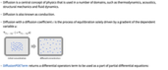
- 扩散是物理学的中心概念,应用于许多领域,如热力学、声学、结构力学和流体动力学等.
- 扩散也称为传导(Conduction).
- 扩散系数为
的扩散是仅由因变量
的梯度驱动的平衡过程: - DiffusionPDETerm 返回微分算子项,该项将用作偏微分方程的一部分:
- DiffusionPDETerm 可用来模拟扩散方程,其中因变量为
,自变量为
,时间变量为
. - 平稳模型变量 vars 为 vars={u[x1,…,xn],{x1,…,xn}}.
- 与时间相关的模型变量 vars 为 vars={u[t,x1,…,xn],{x1,…,xn}} 或 vars={u[t,x1,…,xn],t,{x1,…,xn}}.
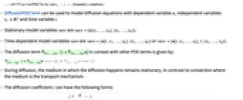
- 与其他偏微分方程项相关的扩散项

由下式给出: - 在扩散过程中,发生扩散的介质保持静止,这与介质作为输送机制的对流相反.
- 扩散系数
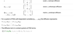
具有以下形式: -


标量
,各向同性扩散{c1,…,cn} 
- 向量
,正交各向异性扩散
{{c11,…,c1n},…,{cn1,…,cnn}} 
- 矩阵
,各向异性扩散
- 向量
- 对于具有因变量 {u1,…,um} 的偏微分方程组,扩散表示:
- 扩散项在相关的偏微分方程组中:
- 扩散系数
是秩为 4 的张量,形如
,其中各子矩阵
为
矩阵,其指定方式与单个因变量的指定方式相同. - 可通过 MatrixSymbol 指定符号扩散系数. »
- 扩散系数
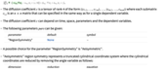
可取决于时间、空间、参数和因变量. - 可以给出以下参数 pars:
-
Italic 参数 默认 符号 "CoordinateChart" "Cartesian" 
"RegionSymmetry" None 
- 参数 "RegionSymmetry" 的一个可能选择为 "Axisymmetric".
- "Axisymmetric" 区域对称性表示截断圆柱坐标系,其中通过移除角度变量来简化圆柱坐标,如下所示:
-
维度 简化 方程式 1D 


2D 

- 系数
影响 NeumannValue 的意义. - 所有不明确依赖于给定自变量的量,其偏导数均被视为零.

范例
打开所有单元 关闭所有单元基本范例 (6)
DiffusionPDETerm[{u[x], {x}}, 1]Activate[%]DiffusionPDETerm[{u[x], {x}}, κ, <|{κ -> {{1}}}|>]Activate[%]DiffusionPDETerm[{u[x], {x}}, {{κ[x]}}]Activate[%]NDEigenvalues[DiffusionPDETerm[{u[x], {x}}], u, {x}∈Line[{{0}, {1}}], 3]vars = {u[x, y], {x, y}};
DSolveValue[Activate[DiffusionPDETerm[vars] == SourcePDETerm[vars, 1]], u[x, y], {x, y}]ufun = NDSolveValue[{D[u[t, x], t] + DiffusionPDETerm[{u[t, x], {x}}, 1] == 0, u[0, x] == Exp[-x ^ 2]}, u, {t, 0, 1}, {x, -π, π}]Plot[Evaluate[Table[ufun[t, x], {t, 0, 1, 0.25}]], {x, -π, π}, Rule[...]]NIntegrate[ufun[0, x], {x, -π, π}] - NIntegrate[ufun[1, x], {x, -π, π}]范围 (36)
一维 (6)
DiffusionPDETerm[{u[t, x], {x}}, MatrixSymbol["c", {1, 1}]]Activate[%]DiffusionPDETerm[{u[x], {x}}]DiffusionPDETerm[{u[t, x], {x}}, {{1 + t}}]Activate[%]κ = MatrixSymbol["c", {1, 1}];
DiffusionPDETerm[{u[x], {x}}, κ, <|{κ -> {{1}}}|>]Activate[%]使用 DiffusionPDETerm 模拟特征值问题:
NDEigensystem[DiffusionPDETerm[{u[x], {x}}, 1], u, {x, 0, 1}, 3]使用 DiffusionPDETerm 建立一维泊松方程:
NDSolveValue[{DiffusionPDETerm[{u[x], {x}}, 1] == 1, DirichletCondition[u[x] == 0, True]}, u, {x, 0, 1}]Plot[%[x], {x, 0, 1}]一维轴对称 (1)
DiffusionPDETerm[{u[r], {r}}, 1, <|"RegionSymmetry" -> "Axisymmetric"|>]将 Activate 应用于该项:
Activate[%]使用构成扩散方程的算子验证轴对称情况是使用截断圆柱坐标系的结果:
Div[-1 * Grad[u[r], {r, θ, z}, "Cylindrical"], {r, θ, z}, "Cylindrical"]二维 (13)
DiffusionPDETerm[{u[x, y], {x, y}}, 1]Activate[%]DiffusionPDETerm[{u[x, y], {x, y}}]DiffusionPDETerm[{u[x, y], {x, y}}, 1] == 0Activate[%]DiffusionPDETerm[{u[x, y], {x, y}}, MatrixSymbol["c", {2, 2}]]Activate[%]D[u[t, x, y]] + DiffusionPDETerm[{u[t, x, y], {x, y}}, 1] == 0Activate[%]DiffusionPDETerm[{u[x, y], {x, y}}, {10, 20}]DiffusionPDETerm[{u[x, y], {x, y}}, {{2, 1}, {0, 1}}]DiffusionPDETerm[{u[t, x, y], t, {x, y}}, {{2, 1}, {0, 1}}]使用 DiffusionPDETerm 建立二维泊松方程:
NDSolveValue[{DiffusionPDETerm[{u[x, y], {x, y}}, 1] == 1, DirichletCondition[u[x, y] == 0, True]}, u, {x, y}∈Rectangle[]]ContourPlot[%[x, y], {x, y}∈Rectangle[]]vars = {u[x, y], {x, y}};
NDSolveValue[{DiffusionPDETerm[vars] == SourcePDETerm[vars, 1], DirichletCondition[u[x, y] == 0, True]}, u[x, y], {x, y}∈Disk[]]Plot3D[%, {x, y}∈Disk[]]使用向量值扩散系数,该系数在
方向的扩散常数大于
方向的扩散常数:
NDSolveValue[{DiffusionPDETerm[{u[x, y], {x, y}}, {10, 1}] == 1, DirichletCondition[u[x, y] == 0, True]}, u, {x, y}∈Rectangle[]]ContourPlot[%[x, y], {x, y}∈Rectangle[]]使用向量值扩散系数,该系数在
方向的扩散常数大于
方向的扩散常数:
NDSolveValue[{DiffusionPDETerm[{u[x, y], {x, y}}, {1, 10}] == 1, DirichletCondition[u[x, y] == 0, True]}, u, {x, y}∈Rectangle[]]ContourPlot[%[x, y], {x, y}∈Rectangle[]]NDSolveValue[{DiffusionPDETerm[{u[x, y], {x, y}}, {{1, 1 / 2}, {1 / 2, 1}}] == 1, DirichletCondition[u[x, y] == 0, True]}, u, {x, y}∈Rectangle[]]ContourPlot[%[x, y], {x, y}∈Rectangle[]]二维轴对称 (3)
DiffusionPDETerm[{u[r, z], {r, z}}, 1, <|"RegionSymmetry" -> "Axisymmetric"|>] == 0将 Activate 应用于项:
Activate[%]使用构成扩散方程的算子验证轴对称情况是使用截断圆柱坐标系的结果:
Div[{{-1, 0, 0}, {0, -1, 0}, {0, 0, -1}}. Grad[u[r, z], {r, θ, z}, "Cylindrical"], {r, θ, z}, "Cylindrical"]D[u[t, r, z]] + DiffusionPDETerm[{u[t, r, z], {r, z}}, 1, <|"RegionSymmetry" -> "Axisymmetric"|>] == 0将 Activate 应用于项:
Activate[%]D[u[t, r, z]] + DiffusionPDETerm[{u[t, r, z], {r, z}}, 1, <|"RegionSymmetry" -> "Axisymmetric"|>] == 0将 Activate 应用于项:
Activate[%]三维 (1)
使用 DiffusionPDETerm 建立三维泊松方程:
usol = NDSolveValue[
{DiffusionPDETerm[{u[x, y, z], {x, y, z}}, -1] == 1,
DirichletCondition[u[x, y, z] == x y z, True]}, u, {x, y, z}∈ Ball[]]DensityPlot3D[usol[x, y, z], {x, y, z}∈Ball[], PlotLegends -> Automatic, AxesLabel -> Automatic]坐标系 (3)
DiffusionPDETerm[{u[r, z], {r, z}}, 1, <|"CoordinateChart" -> "Polar"|>]Activate[%]与 Laplacian 相比较:
Laplacian[u[r, z], {r, z}, "Polar"]{vals, funs} = NDEigensystem[{DiffusionPDETerm[{u[r, θ], {r, θ}}, 1, <|"CoordinateChart" -> "Polar"|>], DirichletCondition[u[r, θ] == 0, r == π], PeriodicBoundaryCondition[u[r, θ], θ == -π && r < π, Function[X, X + {0, 2π}]]}, u, {r, θ}∈Rectangle[{0, -π}, {π, π}], 4]RevolutionPlot3D[#[r, θ], {r, 0, π}, {θ, -π, π}, PlotRange -> All]& /@ funsifun = NDSolveValue[{DiffusionPDETerm[{u[r, θ], {r, θ}}, 1, <|"CoordinateChart" -> "Polar"|>] == 0, DirichletCondition[u[r, θ] == Sin[4 θ], r == 3]}, u, {r, θ}∈Rectangle[{-3, -3}, {3, 3}]]Plot3D[Evaluate[ifun[r, θ] /. {r -> Sqrt[x ^ 2 + y ^ 2], θ -> ArcTan[y / x]}], {x, y}∈Disk[{0, 0}, 3]]耦合 (6)
DiffusionPDETerm[{{u[x], v[x]}, {x}}]DiffusionPDETerm[{{u[x], v[x]}, {x}}, 1]DiffusionPDETerm[{{u[x], v[x]}, {x}}, {{Subscript[c, 11], Subscript[c, 12]}, {Subscript[c, 21], Subscript[c, 22]}}]DiffusionPDETerm[{{u[x, y], v[x, y]}, {x, y}}, {{Subscript[c, 11], {Subscript[c, 1211], Subscript[c, 1222]}}, {0, {{Subscript[c, 2211], Subscript[c, 2212]}, {Subscript[c, 2221], Subscript[c, 2222]}}}}]cIn = Array[Subscript[c, ##]&, {2, 2, 2, 2}]DiffusionPDETerm[{{u[x, y], v[x, y]}, {x, y}}, cIn]MatrixForm[coefficients = {{{{1, 0}, {0, 1}}, {{0, 2}, {2, 0}}}, {{{0, 0}, {0, 0}}, {{1, 0}, {0, 1}}}}]{uif, vif} = NDSolveValue[{DiffusionPDETerm[{{u[x, y], v[x, y]}, {x, y}}, coefficients] == {1, 1}, DirichletCondition[{u[x, y] == 0, v[x, y] == 0}, True]}, {u, v}, {x, y}∈Rectangle[]];GraphicsRow[{ContourPlot[uif[x, y], {x, y}∈Rectangle[]], ContourPlot[vif[x, y], {x, y}∈Rectangle[]]}]耦合轴对称 (3)
使用 DiffusionPDETerm 建立具有多个因变量的一维轴对称方程:
eqn = DiffusionPDETerm[{{u[r], v[r]}, {r}}, {{2.4, 3}, {3, 3}}, <|"RegionSymmetry" -> "Axisymmetric"|>] == {1, 1}bcs = {u[0.1] == 200, v[0.1] == 200, u[0.5] == 50, v[0.5] == 5};{uif, vif} = NDSolveValue[{eqn, bcs}, {u, v}, {r, 0.1, 0.5}]{fufun, fvfun} = DSolveValue[{eqn, bcs}, {u, v}, {r}]Plot[{fufun[r] - uif[r], fvfun[r] - vif[r]}, {r, 0.1, 0.5}, PlotLegends -> "Expressions", PlotRange -> All]DiffusionPDETerm[{{u[r, z], v[r, z]}, {r, z}}, 1, <|"RegionSymmetry" -> "Axisymmetric"|>]将 Activate 应用于项:
Activate[%]MatrixForm[
coefficients = {{{{25, 0}, {0, 25}}, {{0, 10}, {5, 0}}}, {{{0, 15}, {20, 0}}, {{50, 0}, {0, 25}}}}]coupledPDEs = DiffusionPDETerm[{{u[r, z], v[r, z]}, {r, z}}, coefficients, <|"RegionSymmetry" -> "Axisymmetric"|>];{uif, vif} = NDSolveValue[{coupledPDEs == {1, 1}, DirichletCondition[{u[r, z] == 0, v[r, z] == 0}, z == 0]}, {u, v}, {r, z}∈Rectangle[]];GraphicsRow[{ContourPlot[uif[r, z], {r, z}∈Rectangle[]], ContourPlot[vif[r, z], {r, z}∈Rectangle[]]}]应用 (9)
使用带有可变扩散系数的 DiffusionPDETerm:
model = DiffusionPDETerm[{u[x], {x}}, {{If[x ≤ 3 / 4, 1, 2]}}]solution = NDSolveValue[{model == 0, DirichletCondition[u[x] == 1, x == 0], DirichletCondition[u[x] == 0, x == 1]}, u, {x, 0, 1}]flux = model /. Inactive[Div][flux_, _] :> Activate[flux]Plot[Evaluate[{solution[x], flux /. u -> solution}], {x, 0, 1}, ...]将 DiffusionPDETerm 用于轴对称几何对传导热传递进行建模中.
分析区域是二维区域. 除了在笛卡尔坐标
中定义完整的二维区域,您还可以在一维
中定义具有截断圆柱坐标的区域. 因为方程组围绕
轴旋转对称因此柱坐标变量
和
消失.
eqn = DiffusionPDETerm[{u[r], {r}}, 2.4, <|"RegionSymmetry" -> "Axisymmetric"|>] == 0bcs = {u[1 / 10] == 200, u[1 / 2] == 50};numericSolution = NDSolveValue[{eqn, bcs}, u, {r, 0.1, 0.5}]或用 DSolveValue 符号求解:
analytocalSolution = DSolveValue[{eqn, bcs}, u, r]Plot[analytocalSolution[r] - numericSolution[r], {r, 0.1, 0.5}, PlotRange -> All]使用 DiffusionPDETerm 模拟大坝下的物种扩散. 设置区域:
Subscript[Ω, dam] = Rectangle[{6, 3}, {12, 18}];
Subscript[Ω, sediment] = RegionDifference[Rectangle[{0, 0}, {18, 6}], Subscript[Ω, dam]];model = DiffusionPDETerm[{u[x, y], {x, y}}, 10 ^ -4]solution = NDSolveValue[{model == 0, DirichletCondition[u[x, y] == 16, x ≤ 6 && y == 6], DirichletCondition[u[x, y] == 8, x ≥ 12 && y == 6]}, u, {x, y}∈Subscript[Ω, sediment]]flux = model /. Inactive[Div][flux_, _] :> Activate[flux]Show[
...,
VectorPlot[Evaluate[flux /. u -> solution], {x, y}∈Subscript[Ω, sediment], Rule[...]]]op = DiffusionPDETerm[{c[x, y], {x, y}}, 1] + ConvectionPDETerm[{c[x, y], {x, y}}, flux /. u -> solution] + 2 * 10 ^ -5c[x, y];concentration = NDSolveValue[{op == 0,
DirichletCondition[c[x, y] == 100, x ≤ 6 && y == 6], DirichletCondition[c[x, y] == 50, x ≥ 12 && y == 6]
}, c, {x, y}∈Subscript[Ω, sediment]]Show[
...,
ContourPlot[concentration[x, y], {x, y}∈Subscript[Ω, sediment], ...],
VectorPlot[Evaluate[flux /. u -> solution], {x, y}∈Subscript[Ω, sediment], Rule[...]]
]helmholtzModel[vars_, k_] := DiffusionPDETerm[vars, 1] + ReactionPDETerm[vars, k]NDEigenvalues[{helmholtzModel[{u[x, y], {x, y}}, 4]}, u, {x, y}∈Disk[], 5]vars = {u[x, y], {x, y}};
NDSolveValue[{helmholtzModel[vars, 4] == SourcePDETerm[vars, 1], DirichletCondition[u[x, y] == 0, True]}, u[x, y], {x, y}∈Disk[]]Plot3D[%, {x, y}∈Disk[]]将 DiffusionPDETerm 用于轴对称几何对传导热传递进行的建模. 分析区域是一个三维空心圆柱体. 除了在笛卡尔坐标
中定义完整的三维区域,您还可以在二维
中定义具有截断圆柱坐标的区域. 因为方程组围绕
轴旋转对称因此柱坐标变量
消失.
Ω = Rectangle[{0.02, 0}, {0.1, 0.14}];model = DiffusionPDETerm[{u[r, z], {r, z}}, 52, <|"RegionSymmetry" -> "Axisymmetric"|>]solution = NDSolveValue[{model == NeumannValue[5 * 10 ^ 5, r == 0.02 && (0.04 <= z <= 0.1)], DirichletCondition[u[r, z] == 273.15, z == 0 || r == 0.1 || z == 0.14]}, u, {r, z}∈Ω]ContourPlot[solution[r, z], {r, z}∈Ω, ...]Legended[RegionPlot3D[0.02^2 ≤ x^2 + y^2 ≤ 0.1^2 && 0 ≤ PlanarAngle[{0, 0} -> {{0.02, 0}, {x, y}}] ≤ (4 π/3), {x, -0.1, 0.1}, {y, -0.1, 0.1}, {z, 0, 0.14}, ...], BarLegend[...]]使用 DiffusionPDETerm 使用轴对称几何对非线性传导热传递进行建模.
radius = 3;
height = 8;
Ω2D = Rectangle[{0, 0}, {radius, height}];Subscript[k, air] = QuantityMagnitude[ThermodynamicData["Air", "ThermalConductivity"]];flux = 10;
temperature = 10;
model2D = {DiffusionPDETerm[{u[r, z], {r, z}}, (Subscript[k, air] + 10^-3u[r, z]) * IdentityMatrix[2], <|"RegionSymmetry" -> "Axisymmetric"|>] == NeumannValue[flux, r == radius], DirichletCondition[u[r, z] == temperature, z == 0]};measure2D =
AbsoluteTiming[
MaxMemoryUsed[
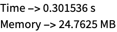
solution2D = NDSolveValue[model2D, u, {r, z}∈Ω2D]]];ContourPlot[solution2D[r, z], {r, z}∈Ω2D, ...]Print["Time -> ", measure2D[[1]], " s", "
Memory -> ", measure2D[[2]] / (1024. ^ 2), " MB"]使用 DiffusionPDETerm 设置平面应力算子. 设置耦合系数:
MatrixForm[coefficients = {{{{(Y/1 - ν^2), 0}, {0, (Y (1 - ν)/2 (1 - ν^2))}}, {{0, (Y ν/1 - ν^2)}, {(Y (1 - ν)/2 (1 - ν^2)), 0}}}, {{{0, (Y (1 - ν)/2 (1 - ν^2))}, {(Y ν/1 - ν^2), 0}}, {{(Y (1 - ν)/2 (1 - ν^2)), 0}, {0, (Y/1 - ν^2)}}}}]model = DiffusionPDETerm[{{u[x, y], v[x, y]}, {x, y}}, coefficients, <|ν -> 1 / 3, Y -> 10 ^ 3|>]Ω = Rectangle[{0, 0}, {5, 1}]{uif, vif} = NDSolveValue[{model == {0, NeumannValue[-1, x == 5]}, DirichletCondition[{u[x, y] == 0., v[x, y] == 0.}, x == 0]}, {u, v}, {x, y}∈Ω]ContourPlot[uif[x, y], {x, y}∈Ω, ...]ContourPlot[vif[x, y], {x, y}∈Ω, ...]flux = model /. Inactive[Div][flux_, _] :> Activate[flux]stokesModel[vars_, μ_] := DiffusionPDETerm[vars, {{μ, 0, 0}, {0, μ, 0}, {0, 0, 0}}] + ConvectionPDETerm[vars, {{0, 0, {1, 0}}, {0, 0, {0, 1}}, {{1, 0}, {0, 1}, 0}}]eqn = stokesModel[{{u[x, y], v[x, y], p[x, y]}, {x, y}}, 1] == {0, 0, 0}Ω = RegionUnion[Rectangle[{0, 0}, {1, 1 / 2}], Rectangle[{1, 1 / 10}, {2, 2 / 5}]];bcs = {DirichletCondition[
{u[x, y] == 4 * 0.3 * y * (0.5 - y) / (0.41) ^ 2, v[x, y] == 0.}, x == 0.], DirichletCondition[{u[x, y] == 0., v[x, y] == 0.}, 0 < x < 2],
DirichletCondition[p[x, y] == 0., x == 2]};{xVel, yVel, pressure} = NDSolveValue[{eqn, bcs}, {u, v, p}, {x, y}∈Ω, Method -> {"FiniteElement", "InterpolationOrder" -> {u -> 2, v -> 2, p -> 1}, "MeshOptions" -> {"MaxCellMeasure" -> 0.0005}}];VectorPlot[{xVel[x, y], yVel[x, y]}, {x, y}∈Ω, AspectRatio -> Automatic, StreamPoints -> 6, StreamColorFunction -> "TemperatureMap", StreamColorFunctionScaling -> False]//Quiet将斯托克斯流模型扩展为纳维-斯托克斯流模型. 定义斯托克斯流模型:
stokesModel[vars_, μ_] := DiffusionPDETerm[vars, {{μ, 0, 0}, {0, μ, 0}, {0, 0, 0}}] + ConvectionPDETerm[vars, {{0, 0, {1, 0}}, {0, 0, {0, 1}}, {{1, 0}, {0, 1}, 0}}]navierStokesModel[vars_, μ_, ρ_] := stokesModel[vars, μ] + ConvectionPDETerm[vars, {{ρ vars[[1, {1, 2}]], 0, 0}, {0, ρ vars[[1, {1, 2}]], 0}, {0, 0, 0}}]eqn = navierStokesModel[{{u[x, y], v[x, y], p[x, y]}, {x, y}}, 1, 10 ^ -3] == {0, 0, 0}Ω = Rectangle[{0, 0}, {1, 1}];bcs = {DirichletCondition[
{u[x, y] == 1, v[x, y] == 0}, y == 1], DirichletCondition[{u[x, y] == 0, v[x, y] == 0}, y < 1],
DirichletCondition[p[x, y] == 0, x == 0 && y == 1]};{xVel, yVel, pressure} = NDSolveValue[{eqn, bcs}, {u, v, p}, {x, y}∈Ω, Method -> {"FiniteElement", "InterpolationOrder" -> {u -> 2, v -> 2, p -> 1}, "MeshOptions" -> {"MaxCellMeasure" -> 0.0005}}];VectorPlot[{xVel[x, y], yVel[x, y]}, {x, y}∈Ω, AspectRatio -> Automatic, StreamPoints -> 6, StreamColorFunction -> "TemperatureMap", StreamColorFunctionScaling -> False]//Quiet属性和关系 (3)
sol1 = NDSolveValue[{DiffusionPDETerm[{u[x, y], {x, y}}, {{1, 1 / 2}, {0, 1}}] == 1, DirichletCondition[u[x, y] == 0, True]}, u, {x, y}∈Rectangle[]]sol2 = NDSolveValue[{DiffusionPDETerm[{u[x, y], {x, y}}, {{1, 1 / 4}, {1 / 4, 1}}] == 1, DirichletCondition[u[x, y] == 0, True]}, u, {x, y}∈Rectangle[]]Plot3D[Chop[sol1[x, y] - sol2[x, y]], {x, y}∈Rectangle[]]nfun = NDSolveValue[{D[u[t, x], t] + DiffusionPDETerm[{u[t, x], {x}}, 1] == 0, DirichletCondition[u[t, x] == 0, True], u[0, x] == Exp[-x ^ 2]}, u[t, x], {t, 0, 1}, {x, -π, π}]afun = DSolveValue[{Activate[D[u[t, x], t] + DiffusionPDETerm[{u[t, x], {x}}, 1] == 0], u[t, -π] == 0, u[t, π] == 0, u[0, x] == Exp[-x ^ 2]}, u, {t, 0, 1}, {x, -π, π}]从 Inactive 和中提取几个项:
asol = afun[t, x] /. {∞ -> 15}//Activate;Plot3D[asol - nfun, {x, -π, π}, {t, 0, 1}, AxesLabel -> {"x", "t"}, PlotRange -> All]ufun = NDSolveValue[{D[u[t, x], t] + DiffusionPDETerm[{u[t, x], {x}}, 1] == 0, DirichletCondition[u[t, x] == 0, True], u[0, x] == 1 / 2 - Abs[x - 1 / 2]}, u, {t, 0, 0.001}, x∈Line[{{0}, {1}}]]Plot[{(1 / 2 - Abs[x - 1 / 2]), ufun[0.001, x]}, {x, 0, 1}, PlotRange -> {{0.35, 0.65}, {0.4, 0.51}}]可能存在的问题 (3)
DiffusionPDETerm[{u[x], {x}}, c]DiffusionPDETerm[{u[x], {x}}, c]DiffusionPDETerm[{u[x], {x}}, c, <|c -> 1|>]DiffusionPDETerm[{u[x], {x}}, c]//Activate数值扩散系数将自动乘以适当大小的 IdentityMatrix:
DiffusionPDETerm[{u[x], {x}}, 1]指定符号矩阵扩散系数的一个方式是通过 MatrixSymbol:
cs = MatrixSymbol["c", {1, 1}];
DiffusionPDETerm[{u[x], {x}}, cs, <|cs -> {{1}}|>]使用 MatrixSymbol 则允许激活算符:
DiffusionPDETerm[{u[x], {x}}, cs]//ActivateDiffusionPDETerm 模拟
,而不是
:
c = 1 / (x + 1);
model = DiffusionPDETerm[{u[x], {x}}, {{c}}];
solution1 = NDSolveValue[{model == 1, DirichletCondition[u[x] == 1, x == 0], DirichletCondition[u[x] == 0, x == 1]}, u, {x, 0, 1}];solution2 = NDSolveValue[{-c Laplacian[u[x], {x}] == 0, DirichletCondition[u[x] == 1, x == 0], DirichletCondition[u[x] == 0, x == 1]}, u, {x, 0, 1}];Plot[{solution1[x], solution2[x]}, {x, 0, 1}, PlotLegends -> {"solution1", "solution2"}]相关指南
-
▪
- 偏微分方程术语
文本
Wolfram Research (2020),DiffusionPDETerm,Wolfram 语言函数,https://reference.wolfram.com/language/ref/DiffusionPDETerm.html (更新于 2026 年).
CMS
Wolfram 语言. 2020. "DiffusionPDETerm." Wolfram 语言与系统参考资料中心. Wolfram Research. 最新版本 2026. https://reference.wolfram.com/language/ref/DiffusionPDETerm.html.
APA
Wolfram 语言. (2020). DiffusionPDETerm. Wolfram 语言与系统参考资料中心. 追溯自 https://reference.wolfram.com/language/ref/DiffusionPDETerm.html 年
BibTeX
@misc{reference.wolfram_2026_diffusionpdeterm, author="Wolfram Research", title="{DiffusionPDETerm}", year="2026", howpublished="\url{https://reference.wolfram.com/language/ref/DiffusionPDETerm.html}", note=[Accessed: 18-July-2026]}
BibLaTeX
@online{reference.wolfram_2026_diffusionpdeterm, organization={Wolfram Research}, title={DiffusionPDETerm}, year={2026}, url={https://reference.wolfram.com/language/ref/DiffusionPDETerm.html}, note=[Accessed: 18-July-2026]}