

FunctionMonotonicity
FunctionMonotonicity[f,x]
变量 x 为实数,求函数 f 的单调性.
FunctionMonotonicity[f,x,dom]
x 被限制在域 dom 内,求 f 的单调性.
FunctionMonotonicity[{f,cons},x,dom]
当 x 别于是条件 cons 限制时给出 f 的单调性.
更多信息和选项
- 单调性亦称为递增、递减、非递增、非递减、严格递增、严格递减.
- 默认情况下,可使用以下定义:
-
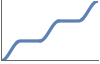
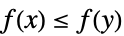
+1 非递减,即对于所有的  ,

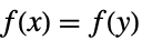
0 恒定,即对于所有的  ,
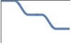
-1 非递增,即对于所有的  ,
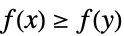
Indeterminate 既不是非递减,也不是非递增 - 常数函数既是非递减,也是非递增的.
- 如果设置 StrictInequalitiesTrue,可使用以下定义:
-
+1 递增,即对于所有的  ,
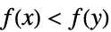
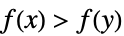
-1 递减,即对于所有的  ,
Indeterminate 既非递减,亦非递增 - dom 的可能的值包括:Reals、Integers、PositiveReals、PositiveIntegers 等. 默认值为 Reals.
- 对于 dom 中满足约束条件 cons 的所有 x,f 应为实值函数.
- cons 可以包含等式、不等式或它们的逻辑组合.
- 可给出以下选项:
-
Assumptions $Assumptions 对参数的设定 GenerateConditions True 是否生成关于参数的条件 PerformanceGoal $PerformanceGoal 优先考虑速度还是质量 StrictInequalities True 是否要求严格单调 - GenerateConditions 的可能的设置包括:
-
Automatic 只给出非通用条件 True 所有条件 False 不给出条件 None 如果需要条件则不经计算直接返回 - PerformanceGoal 的可能设置为 "Speed" 和 "Quality".
范例
打开所有单元 关闭所有单元基本范例 (3)
范围 (5)
FunctionMonotonicity[Sin[x], x]FunctionMonotonicity[2 ^ x, x]FunctionMonotonicity[Sqrt[x ^ 2] - x, x]Plot[{Sin[x], 2 ^ x, Sqrt[x ^ 2] - x}, {x, -3, 3}]非实值函数的单调性为 Indeterminate:
FunctionMonotonicity[Log[x], x]
FunctionMonotonicity[{Log[x], x > 0}, x]FunctionMonotonicity[{Sin[x], -Pi / 2 ≤ x ≤ Pi / 2}, x]FunctionMonotonicity[{Sqrt[x ^ 2] - x, x ≥ 0}, x]FunctionMonotonicity[Floor[x], x, StrictInequalities -> True]FunctionMonotonicity[Floor[x] + x, x, StrictInequalities -> True]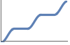

Plot[{Floor[x], Floor[x] + x}, {x, -10, 10}]FunctionMonotonicity[x ^ 3 + a x + b, x]选项 (5)
Assumptions (1)
FunctionMonotonicity 给出有条件的答案:
FunctionMonotonicity[a x + 1, x]
FunctionMonotonicity[a x + 1, x, Assumptions -> a < 0]GenerateConditions (2)
默认情况下,FunctionMonotonicity 可能会对符号参数生成条件:
FunctionMonotonicity[E ^ (a x), x]如果设置 GenerateConditionsNone,FunctionMonotonicity 会失败,而不是给出有条件的结果:
FunctionMonotonicity[E ^ (a x), x, GenerateConditions -> None]FunctionMonotonicity[E ^ (a x), x, GenerateConditions -> False]FunctionMonotonicity[x / a ^ 2, x]如果设置 GenerateConditionsAutomatic,不报告通常为真的条件:
FunctionMonotonicity[x / a ^ 2, x, GenerateConditions -> Automatic]PerformanceGoal (1)
用 PerformanceGoal 避免潜在费时的计算:
FunctionMonotonicity[a x ^ 5 + b x ^ 3 + c x ^ 2 + d x, x, PerformanceGoal -> "Speed"]FunctionMonotonicity[a x ^ 5 + b x ^ 3 + c x ^ 2 + d x, x]StrictInequalities (1)
默认情况下,FunctionMonotonicity 计算的是非严格单调性:
FunctionMonotonicity[#, x]& /@ {Ramp[x] + 1, Ramp[x] + x}如果设置 StrictInequalitiesTrue,FunctionMonotonicity 计算严格单调性:
FunctionMonotonicity[#, x, StrictInequalities -> True]& /@ {Ramp[x] + 1, Ramp[x] + x}Ramp[x]+1 非递减,但不是严格递增. Ramp[x]+x 严格递增:
Plot[{Ramp[x] + 1, Ramp[x] + x}, {x, -2, 2}]应用 (19)
基本应用 (5)


Table[FunctionMonotonicity[f, x, PositiveReals], {f, {x^1 / 3, Sqrt[x], x, x^2, x^3}}]Plot[{x^1 / 3, Sqrt[x], x, x^2, x^3}, {x, 0, 2}, Rule[...]]FunctionMonotonicity[x^α, x, PositiveReals, Assumptions -> α > 0]FunctionMonotonicity[x^α, x, PositiveReals, Assumptions -> α > 0, StrictInequalities -> True]

Table[FunctionMonotonicity[f, x, PositiveReals], {f, {(1/x^1 / 3), (1/Sqrt[x]), (1/x), (1/x^2), (1/x^3)}}]Plot[{(1/x^1 / 3), (1/Sqrt[x]), (1/x), (1/x^2), (1/x^3)}, {x, 0, 2}, PlotLegends -> "Expressions"]FunctionMonotonicity[x^α, x, PositiveReals, Assumptions -> α < 0, StrictInequalities -> True]

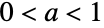
{FunctionMonotonicity[a^x, x, Assumptions -> a > 1], FunctionMonotonicity[a^x, x, Assumptions -> 0 < a < 1]}Plot[{0.5^x, 1.5^x}, {x, -3, 3}]FunctionMonotonicity[Sin[x], x]Plot[Sin[x], {x, -3Pi, 3Pi}]FunctionMonotonicity[{Sin[x], -Pi / 2 ≤ x ≤ Pi / 2}, x]Plot[Sin[x], {x, -Pi / 2, Pi / 2}]
FunctionMonotonicity[Ceiling[x], x]FunctionMonotonicity[Ceiling[x], x, StrictInequalities -> True]Plot[Ceiling[x], {x, -5, 5}]组合函数的情况 (5)


{f, g} = {Cos[x] - x, 5Erfc[x / 5]};{FunctionMonotonicity[f, x], FunctionMonotonicity[g, x]}FunctionMonotonicity[f + g, x]Plot[{f, g, f + g}, {x, -10, 10}, Rule[...]]{f, g} = {Floor[E ^ x], Erf[x] + 1};{FunctionMonotonicity[f, x], FunctionMonotonicity[g, x]}FunctionMonotonicity[f g, x]Plot[{f, g, f g}, {x, -2, 2}, ...]{f, g} = {Function[x, Sinh[x / 3]], Function[x, x + Sin[x]]};{FunctionMonotonicity[f[x], x], FunctionMonotonicity[g[x], x]}{FunctionMonotonicity[f[g[x]], x], FunctionMonotonicity[g[f[x]], x]}Plot[{f[g[x]], g[f[x]]}, {x, -10, 10}, PlotLegends -> "Expressions"]f = Function[x, ConditionalExpression[x ^ 3 - x ^ 2 + x, Element[x, Reals]]]FunctionMonotonicity[f[x], x]g = InverseFunction[f]FunctionMonotonicity[g[x], x]Plot[{f[x], g[x]}, {x, -2, 2}, Rule[...]]

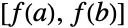
f[x_] := Gamma[x] + Log[x ^ 2]FunctionMonotonicity[{f[x], 1 ≤ x ≤ 5}, x]{f[1], f[5]}为了比较,用 FunctionRange 计算值域:
FunctionRange[{f[x], 1 ≤ x ≤ 5}, x, y]Plot[{f[x], f[1], f[5]}, {x, 1, 5}]微积分 (4)


f = ArcTan[x] + Sin[x] / (2x ^ 2);Plot[f, {x, 1 / 2, 30}, PlotRange -> All]

FunctionMonotonicity[{f, x ≥ 2}, x]FunctionSign[{2 - f, x ≥ 2}, x]


Limit[f, x -> Infinity]MaxValue[{f, x ≥ 2}, x]
f = 2 ^ -n - 3 ^ -n;Plot[f, {n, 1, 10}]FunctionSign[{f, n ≥ 1}, n]s = Sum[f, {n, 1, k}]FunctionMonotonicity[{s, k ≥ 1}, k]FunctionSign[{1 - s, k ≥ 1}, k]用 Sum 计算级数的和:
Sum[f, {n, 1, Infinity}]
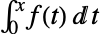

f = t ^ 2 Sin[5t] ^ 4;FunctionSign[f, t]Plot[f, {t, -5, 5}]g = Integrate[f, {t, 0, x}]FunctionMonotonicity[g, x]Plot[g, {x, -5, 5}]f = x ^ 4 - 2x ^ 3 + x;finc = Integrate[Max[D[f, x], 0] + 1, x]//Togetherfdec = Integrate[Min[D[f, x], 0] - 1, x]//Togetherf - (finc + fdec)//Simplify

FunctionMonotonicity[finc, x]FunctionMonotonicity[fdec, x]Plot[{f, finc, fdec}, {x, -1, 2}]概率 (3)
CDF 总是非递减函数:
cdf = CDF[NormalDistribution[], x]FunctionMonotonicity[cdf, x]Plot[cdf, {x, -5, 5}]SurvivalFunction 总是非递增的:
sf = SurvivalFunction[NormalDistribution[], x]FunctionMonotonicity[sf, x]Plot[sf, {x, -5, 5}]Quantile 在  上总是非递减:
qf = Quantile[NormalDistribution[], x]FunctionMonotonicity[{qf, 0 < x < 1}, x]Plot[qf, {x, 0, 1}]解方程和优化 (2)





f[x_] := RiemannR[x ^ 2 + 1] - 2FunctionMonotonicity[{f[x], 0 ≤ x ≤ 3}, x, StrictInequalities -> True, "Continuity" -> True]用 Solve 求根:
Solve[RiemannR[x ^ 2 + 1] - 2 == 0 && 0 ≤ x ≤ 3, x]Plot[f[x], {x, 0, 3}, Epilog -> {Red, Point[{x /. %[[1]], 0}]}]
f[t_] := Erf[t]
g[x_, y_] := x ^ 3 - 5x y + y ^ 3
constraints = x ^ 2 + y ^ 2 ≤ 1;FunctionMonotonicity[f[t], t]
{mval, mpoint} = Maximize[{g[x, y], constraints}, {x, y}]//RootReduce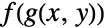


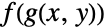
{f[mval], mpoint}Maximize[{f[g[x, y]], constraints}, {x, y}]//RootReduceShow[{Plot3D[{f[g[x, y]], f[mval]}, {x, -1, 1}, {y, -1, 1}, ...], Graphics3D[{Red, PointSize[Large], Point[{x, y, f[mval]} /. mpoint]}]}]属性和关系 (2)
f[x_] := ArcTan[x]
g[x_] := 2 ^ xFunctionMonotonicity[#, x]& /@ {f[x], g[x], f[x] + g[x], f[g[x]], g[f[x]]}Plot[{f[x], g[x], f[x] + g[x], f[g[x]], g[f[x]]}, {x, -2, 2}]f = x ^ 3 - x ^ 2Cos[x] + x Sin[x]FunctionMonotonicity[f, x]用 D 计算导数:
g = D[f, x]用 FunctionSign 验证导数非负:
FunctionSign[g, x]Plot[{f, g}, {x, -7, 7}]文本
Wolfram Research (2020),FunctionMonotonicity,Wolfram 语言函数,https://reference.wolfram.com/language/ref/FunctionMonotonicity.html.
CMS
Wolfram 语言. 2020. "FunctionMonotonicity." Wolfram 语言与系统参考资料中心. Wolfram Research. https://reference.wolfram.com/language/ref/FunctionMonotonicity.html.
APA
Wolfram 语言. (2020). FunctionMonotonicity. Wolfram 语言与系统参考资料中心. 追溯自 https://reference.wolfram.com/language/ref/FunctionMonotonicity.html 年