LogitModelFit[{{x1,y1},{x2,y2},…},{f1,f2,…},x]
constructs a binomial logistic regression model of the form ![]() that fits the yi for each xi.
that fits the yi for each xi.
LogitModelFit[data,{f1,…},{x1,x2,…}]
constructs a binomial logistic regression model of the form ![]() where the fi depend on the variables xk.
where the fi depend on the variables xk.
LogitModelFit[{m,v}]
constructs a binomial logistic regression model from the design matrix m and response vector v.


LogitModelFit
LogitModelFit[{{x1,y1},{x2,y2},…},{f1,f2,…},x]
constructs a binomial logistic regression model of the form ![]() that fits the yi for each xi.
that fits the yi for each xi.
LogitModelFit[data,{f1,…},{x1,x2,…}]
constructs a binomial logistic regression model of the form ![]() where the fi depend on the variables xk.
where the fi depend on the variables xk.
LogitModelFit[{m,v}]
constructs a binomial logistic regression model from the design matrix m and response vector v.
Details and Options


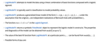
- LogitModelFit attempts to model the data using a linear combination of basis functions composed with a logistic sigmoid.
- LogitModelFit is typically used in classification to model probability values.
- LogitModelFit produces a generalized linear model of the form
 under the assumption that the original
  are independent realizations of Bernoulli trials with probabilities
  .
. - The function
 is the LogisticSigmoid.
 - LogitModelFit returns a symbolic FittedModel object to represent the logistic model it constructs. The properties and diagnostics of the model can be obtained from model["property"].
- The value of the best-fit function from LogitModelFit at a particular point x1, … can be found from model[x1,…].
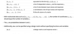
- Possible forms of data are:
-
{y1,y2,…} equivalent to the form {{1,y1},{2,y2},…} {{x11,x12,…,y1},…} a list of independent values xij and the responses yi {{x11,x12,…}y1,…} a list of rules between input values and response {{x11,x12,…},…}{y1,y2,…} a rule between a list of input values and responses {{x11,…,y1,…},…}n fit the n  column of a matrix
Tabular[…]name fit the column name in a tabular object - With multivariate data such as
 , the number of coordinates xi1, xi2, … should equal the number of variables xi.
 - The yi are probabilities between 0 and 1.
- Additionally, data can be specified using a design matrix without specifying functions and variables:
-
{m,v} a design matrix m and response vector v - In LogitModelFit[{m,v}], the design matrix m is formed from the values of basis functions fi at data points in the form {{f1,f2,…},{f1,f2,…},…}. The response vector v is the list of responses {y1,y2,…}.
- For a design matrix m and response vector v, the model is
 , where
  is the vector of parameters to be estimated.
 - When a design matrix is used, the basis functions fi can be specified using the form LogitModelFit[{m,v},{f1,f2,…}].
- LogitModelFit is equivalent to GeneralizedLinearModelFit with ExponentialFamily->"Binomial" and LinkFunction->Automatic.
- LogitModelFit takes the same options as GeneralizedLinearModelFit, with the exception of ExponentialFamily and LinkFunction.
Examples
open all close allBasic Examples (1)
Scope (13)
Data (6)
Fit data with success probability responses, assuming increasing integer-independent values:
Weight by the number of observations for each predictor value:
This gives the same best fit function as success failure data:
Fit a rule of input values and responses:
Specify a column as the response:
Fit a model given a design matrix and response vector:
Properties (7)
Data & Fitted Functions (1)
Residuals (1)
Dispersion and Deviances (1)
Parameter Estimation Diagnostics (1)
Influence Measures (1)
Generalizations & Extensions (1)
Options (8)
ConfidenceLevel (1)
The default gives 95% confidence intervals:
Set the level to 90% within FittedModel:
CovarianceEstimatorFunction (1)
DispersionEstimatorFunction (1)
LinearOffsetFunction (1)
Fit data to a model with a known Sqrt[x] term:
NominalVariables (1)
WorkingPrecision (1)
Use WorkingPrecision to get higher precision in parameter estimates:
Reduce the precision in property computations after the fitting:
Properties & Relations (4)
A default "Binomial" model from GeneralizedLinearModelFit is equivalent to the model for LogitModelFit:
ProbitModelFit is equivalent to a "Binomial" model with "ProbitLink":
LogitModelFit assumes binomially distributed responses:
NonlinearModelFit assumes normally distributed responses:
LogitModelFit will use the time stamps of a TimeSeries as variables:
Rescale the time stamps and fit again:
LogitModelFit acts pathwise on a multipath TemporalData:
Tech Notes
Text
Wolfram Research (2008), LogitModelFit, Wolfram Language function, https://reference.wolfram.com/language/ref/LogitModelFit.html (updated 2025).
CMS
Wolfram Language. 2008. "LogitModelFit." Wolfram Language & System Documentation Center. Wolfram Research. Last Modified 2025. https://reference.wolfram.com/language/ref/LogitModelFit.html.
APA
Wolfram Language. (2008). LogitModelFit. Wolfram Language & System Documentation Center. Retrieved from https://reference.wolfram.com/language/ref/LogitModelFit.html
BibTeX
@misc{reference.wolfram_2025_logitmodelfit, author="Wolfram Research", title="{LogitModelFit}", year="2025", howpublished="\url{https://reference.wolfram.com/language/ref/LogitModelFit.html}", note=[Accessed: 23-April-2026]}
BibLaTeX
@online{reference.wolfram_2025_logitmodelfit, organization={Wolfram Research}, title={LogitModelFit}, year={2025}, url={https://reference.wolfram.com/language/ref/LogitModelFit.html}, note=[Accessed: 23-April-2026]}