








MaxLimit


詳細とオプション
- MaxLimitは上極限としても知られている.
- MaxLimitは,極限の最小の上界を計算し,常に実数値関数について定義される.収束その他の,実際の極限を必要としないその他の漸近的特性の条件を与えるためにしばしば使われる.
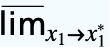
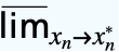
- 最大極値は,記号(
 Mlim
 または\[MaxLimit]で入力)を真下付き文字あるいは下付き文字と一緒に使って次のように入力する.
-
 f
デフォルト方向への最大極限  f
上からの最大極限  f
下からの最大極限  f
複素平面上の最大極限  …
 f
MaxLimit[f,{x1  ,…,xn
 }]
- 有限極限点 x*と{
 ,…,
 }について
-
MaxLimit[f,xx*]f* ![TemplateBox[{{max, (, epsilon, )}, epsilon, 0, +, {Direction, ->, {-, 1}}}, LimitWithSuperscript, DisplayFunction -> ({Sequence[{Sequence["lim"], _, DocumentationBuild`Utils`Private`Parenth[{#2, ->, {#3, ^, DocumentationBuild`Utils`Private`Parenth[#4]}}, LimitsPositioning -> True]}], #1} & ), InterpretationFunction -> ({Limit, [, {#1, ,, {#2, ->, #3}, ,, #5}, ]} & )]=f^*](Files/MaxLimit.ja/24.png "TemplateBox[{{max, (, epsilon, )}, epsilon, 0, +, {Direction, ->, {-, 1}}}, LimitWithSuperscript, DisplayFunction -> ({Sequence[{Sequence[\"lim\"], _, DocumentationBuild`Utils`Private`Parenth[{#2, ->, {#3, ^, DocumentationBuild`Utils`Private`Parenth[#4]}}, LimitsPositioning -> True]}], #1} & ), InterpretationFunction -> ({Limit, [, {#1, ,, {#2, ->, #3}, ,, #5}, ]} & )]=f^*")
MaxLimit[f,{x1,…,xn}{  ,…,
 }]f*
![TemplateBox[{{max, (, epsilon, )}, epsilon, 0, +, {Direction, ->, {-, 1}}}, LimitWithSuperscript, DisplayFunction -> ({Sequence[{Sequence["lim"], _, DocumentationBuild`Utils`Private`Parenth[{#2, ->, {#3, ^, DocumentationBuild`Utils`Private`Parenth[#4]}}, LimitsPositioning -> True]}], #1} & ), InterpretationFunction -> ({Limit, [, {#1, ,, {#2, ->, #3}, ,, #5}, ]} & )]=f^*](Files/MaxLimit.ja/27.png "TemplateBox[{{max, (, epsilon, )}, epsilon, 0, +, {Direction, ->, {-, 1}}}, LimitWithSuperscript, DisplayFunction -> ({Sequence[{Sequence[\"lim\"], _, DocumentationBuild`Utils`Private`Parenth[{#2, ->, {#3, ^, DocumentationBuild`Utils`Private`Parenth[#4]}}, LimitsPositioning -> True]}], #1} & ), InterpretationFunction -> ({Limit, [, {#1, ,, {#2, ->, #3}, ,, #5}, ]} & )]=f^*")
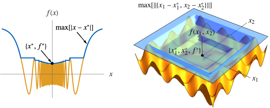
- この定義は,1変量の f[x]についてはmax[ϵ]==MaxValue[{f[x],0<
 <ϵ},x],多変量の f[x1,…,xn]については,最大包絡線max[ϵ]==MaxValue[{f[x1,…,xn],0<
 <ϵ},{x1,…,xn}]を使う.関数max[ϵ]は ϵ0のとき単調減少であるので,常に極限を持つ.この極限は±∞である場合もある.
- 次の図では,max[
 ]とmax[
 ]が青くなっている.
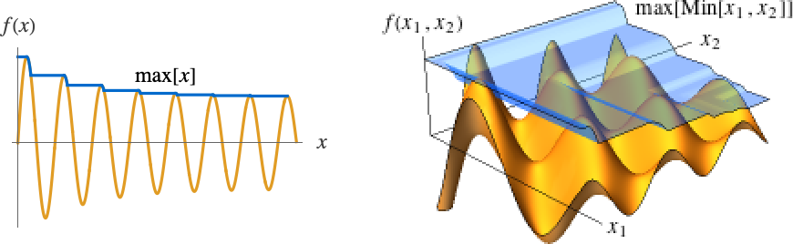
- 無限極限点 x*∞については,1変量の f についてはmax[ω]MaxValue[{f[x],x>ω},x],多変量の f についてはmax[ω]MaxValue[{f[x1,…,xn],x1>ω∧⋯∧xn>ω},{x1,…,xn}]の最大包絡線が使われる.関数max[ω]は ω∞ のとき単調減少なので,常に極限を持つ.
- 次の図ではmax[x]とmax[Min[x1,x2]]が青くなっている.
- 最大極限が求まらなかったとき,MaxLimitは未評価で返される.
- 次は使用可能なオプションである.
-
Assumptions $Assumptions パラメータについての仮定 Direction Reals 極限点に近付く方向 GenerateConditions Automatic パラメータについての条件を生成するかどうか Method Automatic 使用するメソッド PerformanceGoal "Quality" パフォーマンスのどの面について最適化するか - 次はDirectionの可能な設定である.
-
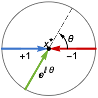
Reals または "TwoSided" 両実数方向から "FromAbove" または -1 上から,つまりより大きい値から "FromBelow" または +1 下から,つまりより小さい値から Complexes すべての複素方向から Exp[ θ]  の方向
{dir1,…,dirn} 方向 diriを変数 xiに独立で使う - x*におけるDirectionExp[ θ]は曲線の接線が極限点 x*に近付く方向を示している.
- 次はGenerateConditionsの可能な設定値である.
-
Automatic 一般的ではない条件のみ True すべての条件 False 条件なし None 条件が必要な場合は未評価で返す - PerformanceGoalの可能な設定には,$PerformanceGoal,"Quality","Speed"がある."Quality"設定のとき,MaxLimitは,一般に,より多くの問題を解いたりより簡単な結果を生成したりするが,より多くの時間とメモリが必要になる可能性がある.
例題
すべて開く すべて閉じる例 (3)
MaxLimit[Sin[x] - 1 / x, x -> ∞]Plot[{Sin[x] - 1 / x, 1}, {x, 0, 30}, PlotStyle -> {Automatic, Dashed}]MaxLimit[(1/x), x -> 0]Plot[(1/x), {x, -1, 1}]MaxLimit[RealAbs[x] / x, x -> 0, Direction -> "FromAbove"]MaxLimit[RealAbs[x] / x, x -> 0, Direction -> "FromBelow"]MaxLimit[RealAbs[x] / x, x -> 0]Plot[RealAbs[x] / x, {x, -1, 1}]スコープ (35)
基本的な用法 (5)
MaxLimit[Sin[x], x -> π / 2]MaxLimit[x / (x - 2a), x -> a]-Infinityにおける最大極限を求める:
MaxLimit[3x ^ 2 / (x ^ 2 - 2), x -> -∞]

MaxLimit[(y/x + y), {y -> 0, x -> 0}]

MaxLimit[(y/x + y), {x -> 0, y -> 0}]
MaxLimit[(y/x + y), {x, y} -> {0, 0}]極限のタイプセット (4)
 Mlim
 を使って 記号を入力し,
 を使って真下付き文字を作る:
Underscript[, x -> 0](x/x^3 + x^2)上付き文字の または
 を極限点の上に使って,上または下からの極限を取る:
Underscript[, x -> 0^ + ](x/x^3 + x^2) を使って上付き文字を作る:
Underscript[, x -> 0^ - ](x/x^3 + x^2)RealsまたはComplexesの方向を指定する際は,記号に真下付き文字として定義域を入れる:
Underscript[, xUnderscript[ -> , ℂ]0]Abs[x]  ->
 で規則を入力し,
 で真下付き文字を作り,
 reals
 とタイプして
 を入力する:
Underscript[, xUnderscript[ -> , ℝ]0]Abs[x]TraditionalFormによる表示:
MaxLimit[f[x], x -> a, Direction -> Reals]//TraditionalForm初等関数 (10)
MaxLimit[a x^2 + b x + c, x -> 2]MaxLimit[4 x ^ 3 - 100x, x -> ∞]MaxLimit[4 x ^ 3 - 100x, x -> -∞]Plot[4 x ^ 3 - 100x + 1, {x, -10, 10}]MaxLimit[(x^2 - 1/x - 1), x -> 1, Direction -> Reals]Plot[{(x^2 - 1/x - 1), 2}, {x, 0, 2}, PlotTheme -> "DashedLines"]MaxLimit[(x^2 + 1/x - 1), x -> 1, Direction -> Reals]Plot[(x^2 + 1/x - 1), {x, 0, 2}, ExclusionsStyle -> Directive[StandardMagenta, Thick, Dashed]]±Infinityにおける有理関数:
MaxLimit[1 / x, x -> ∞]Plot[{1 / x, 0}, {x, -10, 10}, PlotTheme -> "DashedLines", PlotRange -> 1]MaxLimit[(x^2 + 1/2x + 2), x -> ∞]Plot[(x^2 + 1/2x + 2), {x, 0, 10}]MaxLimit[(x^2 + 1/x^2 + 2), x -> -∞]Plot[{(x^2 + 1/x^2 + 2), 1}, {x, -5, 5}, PlotTheme -> "DashedLines"]MaxLimit[CubeRoot[x], x -> -1]MaxLimit[3(x ^ a - a x + a - 1) / (x - 1) ^ 2, x -> 1, Assumptions -> a∈ℝ]MaxLimit[Sqrt[x ^ 2 + 3x] - Sqrt[x ^ 2 + 2x], x -> ∞]Plot[{Sqrt[x ^ 2 + 3x] - Sqrt[x ^ 2 + 2x], 1 / 2}, {x, 0, 20}, PlotRange -> All, PlotTheme -> "DashedLines"]MaxLimit[Tan[x], x -> π / 2]MaxLimit[Tan[x], x -> π / 2, Direction -> "FromAbove"]Plot[Tan[x], {x, 0, Pi}, ExclusionsStyle -> Directive[StandardMagenta, Thick, Dashed]]MaxLimit[Sin[1 / x], x -> 0]Plot[Sin[1 / x], {x, -.1, .1}]±Infinityにおける三角関数:
MaxLimit[Sin[x], x -> ∞]MaxLimit[x Sin[x], x -> ∞]Plot[x Sin[x], {x, 0, 50}]Underscript[, x -> 0](ArcSin[x]/x)Plot[{ArcSin[x] / x, 1}, {x, -1, 1}, PlotTheme -> "DashedLines"]MaxLimit[ArcTan[x ^ 3 - x], x -> ∞]Plot[{ArcTan[x ^ 3 - x], -Pi / 2, Pi / 2}, {x, -5, 5}, PlotTheme -> "DashedLines"]MaxLimit[Exp[(1/x)], x -> 0]Plot[Exp[1 / x], {x, -5, 5}]MaxLimit[(25 ^ x - 5 ^ x) / (4 ^ x - 2 ^ x), x -> 0]//SimplifyPlot[(25 ^ x - 5 ^ x) / (4 ^ x - 2 ^ x), {x, -1, 1}, PlotRange -> {-5, 5}]MaxLimit[x ^ (1 / x), x -> ∞]Plot[{x ^ (1 / x), 1}, {x, 0, 40}, PlotRange -> All, PlotTheme -> "DashedLines"]//QuietMaxLimit[Log[x ^ 2] / x, x -> 0]Plot[Log[x ^ 2] / x, {x, -1, 1}, ExclusionsStyle -> Directive[StandardMagenta, Thick, Dashed]]MaxLimit[x Log[x ^ 2], x -> 0]Plot[Log[x ^ 2]x, {x, -1, 1}]MaxLimit[Log[x] / Sqrt[2x], x -> ∞]Plot[{Log[x] / Sqrt[x], 0}, {x, 0, 1000}, PlotTheme -> "DashedLines", PlotRange -> 1]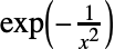


MaxLimit[x^n Exp[-1 / x^2], x -> 0, Assumptions -> n∈ℤ]

MaxLimit[x^n Exp[1 / x^2], x -> 0, Assumptions -> n∈ℤ]Plot[{x^-7 Exp[-x^-2], x^7 Exp[x^-2]}, {x, -1, 1}, PlotRange -> {-5, 5}]区分関数 (5)
f[x_] := Piecewise[{{1, x == 1}}, (x - 1) / (x ^ 2 - 1)]MaxLimit[f[x], x -> 1]f[1]Plot[f[x], {x, 0, 2}, Epilog -> {PointSize[Medium], Point[{1, f[1]}]}]g[x_] := Piecewise[{{1 - x ^ 2, x ≤ 0}}, x ^ 2]MaxLimit[g[x], x -> 0, Direction -> "FromAbove"]MaxLimit[g[x], x -> 0, Direction -> "FromBelow"]MaxLimit[g[x], x -> 0, Direction -> Reals]Plot[g[x], {x, -1, 1}, Epilog -> {PointSize[Medium], Point[{0, g[0]}]}]UnitStepは,事実上,右連続区分関数である:
MaxLimit[UnitStep[x], x -> 0, Direction -> "FromBelow"]MaxLimit[UnitStep[x], x -> 0, Direction -> "FromAbove"]MaxLimit[UnitStep[x], x -> 0]Plot[UnitStep[x], {x, -1, 1}, Epilog -> {ColorData["DefaultPlotColors"][1], PointSize[Large], Point[{0, UnitStep[0]}]}]RealSignは,事実上,不連続区分関数である:
MaxLimit[RealSign[x], x -> 0, Direction -> "FromBelow"]MaxLimit[RealSign[x], x -> 0, Direction -> "FromAbove"]MaxLimit[RealSign[x], x -> 0, Direction -> Reals]
RealSign[0]Plot[RealSign[x], {x, -1, 1}, Epilog -> {ColorData["DefaultPlotColors"][1], PointSize[Medium], Point[{0, RealSign[0]}]}]x が整数値に近付くときのFloorの最大極限を求める:
MaxLimit[Floor[x], x -> n, Assumptions -> n∈Integers]Plot[Floor[x], {x, -4, 4}, ExclusionsStyle -> Dashed]特殊関数 (4)
Gammaを含む上限:
MaxLimit[Gamma[z], z -> -1]MaxLimit[Sin[x]Gamma[x + 1] ^ (1 / x) / x, x -> ∞]Plot[{Sin[x]Gamma[x + 1] ^ (1 / x) / x, 1 / E}, {x, 0, 30}, PlotTheme -> "DashedLines"]MaxLimit[BesselK[1, 3x], x -> 0, Direction -> "FromAbove"]Plot[BesselK[1, 3x], {x, 0, 1}, PlotRange -> {0, 20}]MaxLimit[x SphericalBesselJ[1, 2x], x -> ∞]Plot[{x SphericalBesselJ[1, 2x], 1 / 2}, {x, 0, 10}, PlotTheme -> "DashedLines"]MaxLimit[SquareWave[x]FresnelS[x] / x ^ 3//PiecewiseExpand, x -> 0]Plot[{SquareWave[x]FresnelS[x] / x ^ 3, Pi / 6}, {x, -2, 2}, PlotTheme -> "DashedLines", ExclusionsStyle -> Directive[StandardMagenta, Dashed]]MaxLimit[Cos[x]Erfc[x], x -> -∞]Plot[{Cos[x]Erfc[x], 2}, {x, -28, 2}, PlotStyle -> {Automatic, Dashed}]非正の各偶数で,Gammaは片側から に発散する:
MaxLimit[Gamma[z], z -> a, Assumptions -> a∈ℤ && a ≤ 0 && Mod[a, 2] == 0]MaxLimit[Gamma[z], z -> a, Assumptions -> a∈ℤ && a ≤ 0 && Mod[a, 2] == 1]ネストした最大極限 (3)


MaxLimit[ArcTan[y / x], {y -> ∞, x -> ∞}]2つのMaxLimit式を計算しても同じ結果が得られる:
MaxLimit[MaxLimit[ArcTan[y / x], x -> ∞], y -> ∞]

MaxLimit[ArcTan[y / x], {x -> ∞, y -> ∞}]MaxLimit[MaxLimit[ArcTan[y / x], y -> ∞], x -> ∞]


MaxLimit[Exp[(2y x/Sqrt[1 + y^2x^2 ])], {y -> -∞, x -> 0}]


MaxLimit[Exp[(2y x/Sqrt[1 + y^2x^2 ])], {x -> 0, y -> -∞}]f[x_, y_] := (y /x + y )


MaxLimit[f[x, y], {y -> 0, x -> 0}]


MaxLimit[f[x, y], {x -> 0, y -> 0}] がほとんど
 と相殺し合う点で任意の大きい値が与えられるので,真の二変量最大極限は
 である:
MaxLimit[f[x, y], {x, y} -> {0, 0}]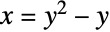
Limit[f[y^2 - y, y], y -> 0, Direction -> "FromAbove"]Show[Plot3D[f[x, y], {x, y}∈Disk[{0, 0}, 2], ClippingStyle -> None, Mesh -> None, BoxRatios -> 1], ParametricPlot3D[{{t, 0, f[t, 0]}, None, {0, t, f[0, t]}}, {t, -2, 2}, PlotStyle -> Thickness[0.025], PlotLegends -> LineLegend[{y == 0, None, x == 0}]], ViewPoint -> {-3, 1, 1}]多変量最大極限 (4)
f[x_, y_] := ArcTan[y ^ 2 / (x ^ 2 + x ^ 3)]MaxLimit[f[x, y], {x -> 0, y -> 0}]MaxLimit[f[x, y], {y -> 0, x -> 0}]
MaxLimit[f[x, x], x -> 0]MaxLimit[f[x, -x], x -> 0]
MaxLimit[f[x, y], {x, y} -> {0, 0}]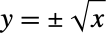
Limit[f[x, Sqrt[x]], x -> 0, Direction -> "FromAbove"]Show[Plot3D[f[x, y], {x, -1, 1}, {y, -1, 1}, Mesh -> None], ParametricPlot3D[{{t^2, t, f[t^2, t]}, None, {t, 0, f[t, 0]}}, {t, -1, 1}, PlotStyle -> Tube[0.05]]]f[x_, y_] := Tanh[(x + y/x - y)]
MaxLimit[Tanh[(x + y/x - y)], {x, y} -> {0, 0}]MaxLimit[f[x, y], {y -> 0, x -> 0}]MaxLimit[Tanh[(x + y/x - y)], {x -> 0, y -> 0}]
f[x, m x]//Simplify最大値には,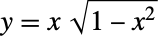 のような
 が
 に近付く曲線に沿って達することができる:
Limit[f[x, xSqrt[1 - x^2]], x -> 0]Show[Plot3D[f[x, y], {x, -1, 1}, {y, -1, 1}, Mesh -> None], ParametricPlot3D[{{t, t Sqrt[1 - t^2], f[t, t Sqrt[1 - t^2]]}, {t, 0, f[t, 0]}, {0, t, f[0, t]}}, {t, -1, 1}, PlotStyle -> Thickness[0.025], PlotLegends -> LineLegend[{y == x Sqrt[1 - x ^ 2], y == 0, x == 0}]], BoxRatios -> Automatic]//Quietf[x_, y_] := (1 + x y)Sin[1 / (x ^ 2 + y ^ 2)]
MaxLimit[f[x, y], {x, y} -> {0, 0}]//Quiet{x[r_, θ_], y[r_, θ_]} := {r Cos[θ], r Sin[θ]};Simplify[f[x[r, θ], y[r, θ]]]極表現は有界で, となるときに消失し,Sinの最大極限を残す:
MaxLimit[f[x[r, θ], y[r, θ]], r -> 0, Direction -> "FromAbove"]ParametricPlot3D[{x[r, θ], y[r, θ], f[x[r, θ], y[r, θ]]}, {r, 0, 1}, {θ, 0, 2Pi}]f[x_, y_, z_] := (x z/x^2 + y^2 + z^2)
MaxLimit[f[x, y, z], {x, y, z} -> {0, 0, 0}]{MaxLimit[f[x, y, z], {x -> 0, y -> 0, z -> 0}], MaxLimit[f[x, y, z], {y -> 0, z -> 0, x -> 0}], MaxLimit[f[x, y, z], {z -> 0, x -> 0, y -> 0}]}

Limit[f[x, 0, x], x -> 0]TransformedField["Cartesian" -> "Spherical", f[x, y, z], {x, y, z} -> {r, θ, φ}]//TrigExpandMaximize[Cos[θ] Cos[φ] Sin[θ], {θ, φ}∈Rectangle[{0, -Pi}, {Pi, Pi}]]//FullSimplify//QuietSliceContourPlot3D[f[x, y, z], {x, y, z}∈Ball[]]オプション (10)
Assumptions (1)
Assumptionsを使ってパラメータについての条件を指定する:
MaxLimit[Sin[x]Exp[a x], x -> ∞, Assumptions -> a < 0]MaxLimit[Sin[x]Exp[a x], x -> ∞, Assumptions -> a == 0]MaxLimit[Sin[x]Exp[a x], x -> ∞, Assumptions -> a > 0]Direction (5)
MaxLimit[1 / x, x -> 0, Direction -> "FromBelow"]MaxLimit[1 / x, x -> 0, Direction -> 1]MaxLimit[1 / x, x -> 0, Direction -> "FromAbove"]MaxLimit[1 / x, x -> 0, Direction -> -1]デフォルトの方向はRealsである:
MaxLimit[1 / x, x -> 0]MaxLimit[1 / x, x -> 0, Direction -> Reals]"TwoSided"はRealsに等しい:
MaxLimit[1 / x, x -> 0, Direction -> "TwoSided"]MaxLimit[Re[-(1/x^2)], x -> 0, Direction -> ℂ]MaxLimit[Re[-(1/x^2)], x -> 0]MaxLimit[-Im[EllipticK[2 + x]], x -> 0, Direction -> +I]MaxLimit[-Im[EllipticK[2 + x]], x -> 0, Direction -> Reals]MaxLimit[-Im[EllipticK[2 + x]], x -> 0, Direction -> -I]f[x_, y_] := (x y/x + y)(2 + RealSign[ x y] + RealSign[y])MaxLimit[f[x, y], {x, y} -> {0, 0}, Direction -> "FromAbove"]MaxLimit[f[x, y], {x, y} -> {0, 0}, Direction -> {"FromAbove", "FromAbove"}]MaxLimit[f[x, y], {x, y} -> {0, 0}, Direction -> {"FromBelow", "FromAbove"}]MaxLimit[f[x, y], {x, y} -> {0, 0}, Direction -> {"FromBelow", Reals}]//QuietMaxLimit[f[x, y], {x, y} -> {0, 0}, Direction -> {Reals, "FromBelow"}]Row@{Plot3D[f[x, y], {x, y}∈Disk[], Exclusions -> {{x == -y , x <= 0}}, ClippingStyle -> None, ImageSize -> 200], DensityPlot[f[x, y], {x, -1, 1}, {y, -1, 1}, Exclusions -> {{x == -y , x <= 0}}, ClippingStyle -> Automatic, ImageSize -> Small]}GenerateConditions (3)
MaxLimit[Sin[x]x ^ n, x -> ∞, GenerateConditions -> False]MaxLimit[Sin[x]x ^ n, x -> ∞]MaxLimit[Cos[x]Exp[a x], x -> ∞, GenerateConditions -> None]デフォルトで,一意的な結果が返されるような条件が生成される:
MaxLimit[Cos[x]Exp[a x], x -> ∞]デフォルトで,特別な値が結果を無効にする場合にのみ条件は生成されない:
MaxLimit[(x y/(x - a)^2 + y^2), {x, y} -> {0, 0}]GenerateConditions->Trueのときは,これらの一般的ではない条件さえも報告される:
MaxLimit[(x y/(x - a)^2 + y^2), {x, y} -> {0, 0}, GenerateConditions -> True]PerformanceGoal (1)
PerformanceGoalを使って,高くつく可能性がある計算を回避する:
expr = (2 y z^2 - z^3 + y (x - 2 y + 3 z)^2 - z (x - 2 y + 3 z)^2/y^2 - 2 y z + z^2 - y (x - 2 y + 3 z) + z (x - 2 y + 3 z) + (x - 2 y + 3 z)^2);MaxLimit[expr, {x, y, z} -> {0, 0, 0}, PerformanceGoal -> "Speed"]デフォルト設定では,使用可能なすべてのテクニックを使って結果を出そうとする:
MaxLimit[expr, {x, y, z} -> {0, 0, 0}]アプリケーション (13)
最大極限の幾何学 (3)


f[x_] := Cos[Log[RealAbs[x]]] + Sin[x]MaxLimit[f[x], x -> 0, Direction -> Reals]このことは, のときに
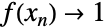 である数列
 (例えば
 )がなければならないことを意味する:
x[n_] := Exp[-2n Pi]
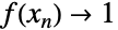
TableForm[N[Table[{x[n], f[x[n]]}, {n, 1, 5}], 10], TableHeadings -> {{}, {Subscript[x, n], HoldForm@f[Subscript[x, n]]}}]DiscreteLimit[x[n], n -> ∞]DiscreteLimit[f[x[n]], n -> ∞]この数列は, それ自身が
 のときに極限を持たなくても存在する点に注意のこと:
Limit[f[x], x -> 0]


g[x_] := Cos[x]Sin[Tan[x]]Limit[g[x], x -> Pi / 2]MaxLimit[g[x], x -> Pi / 2] の周りの徐々に小さくなる領域では,
 は徐々に平らになりグラフの中で
 の下になる部分が多くなる:
Manipulate[Plot[{g[x], 0}, {x, Pi / 2 - a, Pi / 2 + a}, PlotRange -> {-.5, 1}, PlotTheme -> "DashedLines"], {a, 1, 0.001}, SaveDefinitions -> True]


f[x_] := Sin[Tan[x]] + (x - Pi / 2)Limit[f[x], x -> Pi / 2]
MaxLimit[f[x], x -> Pi / 2] の周りの徐々に小さくなる領域では,
 は激しく振動するが,
 はどんどんそのよい天井になる:
Manipulate[Plot[{f[x], 1}, {x, Pi / 2 - a, Pi / 2 + a}, PlotTheme -> "DashedLines"], {a, 1, 0.001}, SaveDefinitions -> True]漸近線の解析 (3)
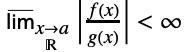 のとき,関数
 は
 における「big-o of
 」(
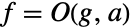 と書く)と言われる:
bigO[x_, a_][f_, g_] := Underscript[, xUnderscript[ -> , ℝ]a]Abs[(f/g)] < ∞

bigO[x, 0][Sin[x], x]
bigO[x, 0][Sin[x], x^2]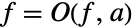
bigO[x, a][f[x], f[x]]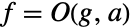
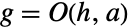
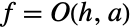
f[x_] := 4x ^ 3 + x ^ 4
g[x_] := x ^ 2 + 4x ^ 3
h[x_] := 3x + 2x ^ 2
{bigO[x, 0][f[x], g[x]], bigO[x, 0][g[x], h[x]], bigO[x, 0][f[x], h[x]]}f[x_] := Piecewise[{{-x, x <= 0}, {1/x, True}}]{bigO[x, 0][1, f[x]], bigO[x, 0][f[x], 1]}
funs = {x ^ 2, 1, x, x Log[x], Sin[x]};

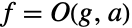
Sort[funs, bigO[x, 0]]テイラー(Taylor)の公理より, が
 の周りに
 個の連続導関数を持つなら
 である:
f[x_] := Exp[x]
t[n_, a_][x_] := Sum[(D[f[x], {x, k}] / k! /. x -> a)(x - a)^k, {k, 0, n}]
t[5, 1][x]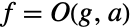
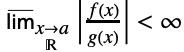
bigO[x_, a_][f_, g_] := Underscript[, xUnderscript[ -> , ℝ]a]Abs[(f/g)] < ∞
bigO[x, 1][f[x] - t[5, 1][x], (x - Pi)^6]DSolveValue[m x''[t] + k x[t] == α Sin[Sqrt[k / m]t], x[t], t, Assumptions -> k > 0 && m > 0]動作は振動していて,任意に大きくなり,不安定さを示している:
MaxLimit[%, t -> ∞, Assumptions -> k > 0 && m > 0]DSolveValue[m x''[t] + β x'[t] + k x[t] == α Sin[Sqrt[k / m]t], x[t], t, Assumptions -> k > 0 && m > 0 && β > 0 && β ^ 2 > 4 k m]振動動作は有界で,徐々に に制限される.これは安定性を示している:
MaxLimit[%, t -> ∞, Assumptions -> k > 0 && m > 0 && β > 0 && β ^ 2 > 4k m]MinLimit[%%, t -> ∞, Assumptions -> k > 0 && m > 0 && β > 0 && β ^ 2 > 4k m]連続性 (4)
 なら,関数は
 において上半連続である.UnitStepは原点において上半連続である:
MaxLimit[UnitStep[x], x -> 0] ≤ UnitStep[0]Plot[UnitStep[x], {x, -1, 1}, PlotStyle -> Thick, Epilog -> {ColorData["DefaultPlotColors"][1], PointSize[Large], Point[{0, UnitStep[0]}]}]一方,RealSignは原点において上半連続ではない:
MaxLimit[RealSign[x], x -> 0] ≤ RealSign[0]Plot[RealSign[x], {x, -1, 1}, PlotStyle -> Thick, Epilog -> {ColorData["DefaultPlotColors"][1], PointSize[Large], Point[{0, RealSign[0]}]}]f[x_] := Piecewise[{{Sin[1/x], x > 0 || x < 0}, {1, x == 0}}]MaxLimit[f[x], x -> 0] ≤ f[0]これは,fが原点において左側極限も右側極限も持たないにもかかわらず,である:
{Underscript[, x -> 0^ + ]f[x], Underscript[, x -> 0^ - ]f[x]}fのMaxLimitは零点におけるfの値に依存しないので,1より大きい任意の値でfが上半連続になる点に注意のこと:
MaxLimit[Piecewise[{{Sin[1/x], x > 0 || x < 0}, {a, x == 0}}], x -> 0]Plot[f[x], {x, -1, 1}, Epilog -> {ColorData["DefaultPlotColors"][2], PointSize[Large], Point[{0, f[0]}]}] (
 )のとき,関数は
 において下(または上)半連続である.実数値関数は,上半連続かつ下半連続のときかつそのときに限り連続である.UnitStepは
 において上半連続である:
MaxLimit[UnitStep[x], x -> 0] ≤ UnitStep[0]MinLimit[UnitStep[x], x -> 0] ≥ UnitStep[0]一方,以下はTriangleWaveが原点で連続であることを示している:
Underscript[, x -> 0]TriangleWave[x] ≤ TriangleWave[0] && Underscript[, x -> 0]TriangleWave[x] ≥ TriangleWave[0]GraphicsRow[Plot[#[x], {x, -1.5, 1.5}, IconizedObject[«Plot options»]]& /@ {UnitStep, TriangleWave}, ImageSize -> Medium]Floorは不連続ではあるがすべての整数で上半連続である:
Table[MaxLimit[Floor[x], x -> k] ≤ Floor[k], {k, -5, 5}]一方,Ceilingは連続でも整数で上半連続でもない:
Table[MaxLimit[Ceiling[x], x -> k] ≤ Ceiling[k], {k, -5, 5}]どちらも非整数値では連続であるが,Floorだけがすべての で上半連続である:
GraphicsRow[{Plot[Floor[x], {x, -5, 5}, IconizedObject[«Plot options»]], Plot[Ceiling[x], {x, -5, 5}, IconizedObject[«Plot options»]]}, ImageSize -> Medium]微分 (3)

diniLU[f_, x_] := Underscript[, h -> 0^ - ]DifferenceQuotient[f, {x, h}]
diniRU[f_, x_] := Underscript[, h -> 0^ + ]DifferenceQuotient[f, {x, h}]Rampは実線全体の上に有限上ディニ微分を持つ:
diniLU[Ramp[x], x]diniRU[Ramp[x], x]これらの2つの微分は原点以外あらゆるところで等しいことに注意のこと:
Simplify[% == %%]これは,Rampは原点以外のあらゆるところで微分可能であることを反映している:
Ramp'[x]Plot[{Ramp[x], Ramp'[x]}, {x, -2, 2}, PlotTheme -> "DashedLines"]f[x_] := Piecewise[{{x*Cos[1/x], x != 0}, {0, True}}]{f[0], Underscript[, xUnderscript[ -> , ℝ]0]f[x]}{Underscript[, h -> 0^ + ](f[h] - f[0]/h), Underscript[, h -> 0^ + ](f[h] - f[0]/h)}{Underscript[, h -> 0^ + ](f[h] - f[0]/h), Underscript[, h -> 0^ + ](f[h] - f[0]/h)}このことは,0の周りの関数の成長が有界であることを示している:
Plot[{f[x], RealAbs[x]}, {x, -1, 1}, PlotTheme -> "DashedLines", Filling -> {1 -> {2}}]右ディニ微分は2つある.最初のものは右上ディニ微分  で,次のように定義される:
diniRU[f_, x_] := Underscript[, h -> 0^ + ]DifferenceQuotient[f, {x, h}]
diniRL[f_, x_] := Underscript[, h -> 0^ + ]DifferenceQuotient[f, {x, h}] は,
 におけるRampと同じように,2つが等しく有限であるときかつそのときに限り,
 で右微分可能である:
{diniRU[Ramp[x], x], diniRL[Ramp[x], x] } /. x -> 0
g[x_] := Piecewise[{{x*Cos[Cot[x]], x != 0}, {0, True}}]{diniRU[g[x], x], diniRL[g[x], x] } /. x -> 0Plot[{Ramp[x], g[x]}, {x, -.1, .1}, PlotTheme -> "DashedLines"]特性と関係 (13)
MaxLimit[x Sin[x], x -> ∞]Limit[x Sin[x], x -> ∞]f[x_] := Sin[x]c = 3;MaxLimit[c f[x], x -> a] == c MaxLimit[f[x], x -> a]


f[x_] := Sin[x]g[x_] := Cos[x]MaxLimit[f[x] + g[x], x -> ∞] ≤ MaxLimit[f[x], x -> ∞] + MaxLimit[g[x], x -> ∞]MaxLimit[f[x] + g[x], x -> ∞] < MaxLimit[f[x], x -> ∞] + MaxLimit[g[x], x -> ∞]Assumptionsは最大極限式でパラメータに適用される:
MaxLimit[Tan[x], x -> π / 2 + n π, Direction -> "FromAbove", Assumptions -> n∈Integers]Directionは極限変数に条件を置く:
MaxLimit[Tan[x], x -> π / 2 + n π, Direction -> "FromBelow", Assumptions -> n∈Integers]Plot[Tan[x], {x, -2π, 2π}, ExclusionsStyle -> {{Dashed, StandardMagenta}}]ネストした最大極限を計算するときは,適切な仮定が後ろの極限変数に対して生成される:
MaxLimit[ArcTan[y / x], {y -> 0, x -> 0}, Direction -> 1]MaxLimit[ArcTan[y / x], x -> 0, Direction -> 1]MaxLimit[ArcTan[y / x], x -> 0, Direction -> 1, Assumptions -> y < 0]実数値関数については,Limitが存在するならMaxLimitは同じ値を持つ:
f[x_] := Sin[x] / xLimit[f[x], x -> ∞]MaxLimit[f[x], x -> ∞]


f[x_] := x / (x + 1)g[x_] := Cos[x]Limit[f[x], x -> ∞]MaxLimit[f[x] + g[x], x -> ∞] == MaxLimit[f[x], x -> ∞] + MaxLimit[g[x], x -> ∞]MaxLimit[SquareWave[x], x -> ∞] ≥ MinLimit[SquareWave[x], x -> ∞]MaxLimitとMinLimitが等しいときは,共通値に等しい極限が存在する:
f[x_] := Piecewise[{{1 + x, x <= 0}, {(x - 1)^2, True}}]{Underscript[, x -> 0]f[x], Underscript[, x -> 0]f[x], Underscript[, x -> 0]f[x]}

{MaxLimit[x, x -> -∞], MinLimit[x, x -> -∞], Limit[x, x -> -∞]}MaxLimitは-MinLimit[-f,…]として計算することができる:
f[x_] := Piecewise[{{2, x > 0}, {-1, True}}]MaxLimit[f[x], x -> 0] == -MinLimit[-f[x], x -> 0]
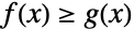

f[x_] := x Sin[1 / x]g[x_] := -RealAbs[x]Reduce[f[x] ≥ g[x]]//SimplifyUnderscript[, xUnderscript[ -> , ℝ]0]f[x] ≤ Underscript[, xUnderscript[ -> , ℝ]0]f[x] ≤ Underscript[, xUnderscript[ -> , ℝ]0]g[x]例のように2つの最大極限が等しいとき, は
 のとき極限を持つ:
Underscript[, xUnderscript[ -> , ℝ]0]f[x] == Underscript[, xUnderscript[ -> , ℝ]0]g[x] == Underscript[, xUnderscript[ -> , ℝ]0]f[x]これは,はさみうちの定理 (またはサンドイッチ定理)の一般化である:
Plot[{f[x], g[x]}, {x, -1, 1}, Filling -> {2 -> {1}}]MaxLimitは常にDiscreteMaxLimit以上である:
g[n_] := Sin[n π + Pi / 4]DiscreteMaxLimit[g[n], n -> ∞]MaxLimit[g[n], n -> ∞]Show[Plot[{g[n], 1, 1 / Sqrt[2]}, {n, 0, 10}, PlotTheme -> "DashedLines"], DiscretePlot[g[n], {n, 0, 10}, PlotMarkers -> {"Point", Medium}]]考えられる問題 (1)

おもしろい例題 (1)
f[x_] := {1 / x ^ 2, Sin[8x] / (6x), 3x ^ 4 / (x ^ 4 + 4), E ^ x, Sin[30 / x], x ^ 2Cos[4x ^ 2] / (x ^ 2 + 1)}a = {0, ∞, ∞, ∞, 0, ∞};range = {{0, 5}, {-0.5, 1.5}, {-2, 4}, {0, 25}, {-2, 2}, {-2, 2}};asym = {6Sign[x + 0.05], 0.02, 3, 0, {-1, 1}, {-1, 1}};Grid[Partition[Table[With[{r1 = f[x][[n]], r2 = a[[n]], r3 = range[[n]], r4 = asym[[n]]},
Plot[{r1, r4}, {x, -4, 4}, PlotRange -> r3, ImageSize -> 210, PlotStyle -> {Automatic, {ThemeColor["Foreground"], Dashed}, {ThemeColor["Foreground"], Dashed}}, ExclusionsStyle -> {{ThemeColor["Foreground"], Dashed}}, PlotLabel -> Style[HoldForm[MaxLimit[r1, x -> r2, Direction -> Reals]] == MaxLimit[f[x][[n]], x -> r2], ScriptLevel -> 0]]], {n, 1, 6}], 2], Frame -> All]テキスト
Wolfram Research (2017), MaxLimit, Wolfram言語関数, https://reference.wolfram.com/language/ref/MaxLimit.html.
CMS
Wolfram Language. 2017. "MaxLimit." Wolfram Language & System Documentation Center. Wolfram Research. https://reference.wolfram.com/language/ref/MaxLimit.html.
APA
Wolfram Language. (2017). MaxLimit. Wolfram Language & System Documentation Center. Retrieved from https://reference.wolfram.com/language/ref/MaxLimit.html