


MaxLimit
Details and Options
- MaxLimit is also known as limit superior, supremum limit, limsup, upper limit and outer limit.
- MaxLimit computes the smallest upper bound for the limit and is always defined for real-valued functions. It is often used to give conditions of convergence and other asymptotic properties where no actual limit is needed.
- By using the character , entered as
 Mlim
Mlim or \[MaxLimit], with underscripts or subscripts max limits can be entered as follows:
 -
 f
fmax limit in the default direction  f
fmax limit from above  f
fmax limit from below  f
fmax limit in the complex plane  …
… f
fMaxLimit[f,{x1  ,…,xn
,…,xn }]
}] - For a finite limit point x* and {
 ,…,
,…, }:
}: -
MaxLimit[f,xx*]f* ![TemplateBox[{{max, (, epsilon, )}, epsilon, 0, +, {Direction, ->, {-, 1}}}, LimitWithSuperscript, DisplayFunction -> ({Sequence[{Sequence["lim"], _, DocumentationBuild`Utils`Private`Parenth[{#2, ->, {#3, ^, DocumentationBuild`Utils`Private`Parenth[#4]}}, LimitsPositioning -> True]}], #1} & ), InterpretationFunction -> ({Limit, [, {#1, ,, {#2, ->, #3}, ,, #5}, ]} & )]=f^* TemplateBox[{{max, (, epsilon, )}, epsilon, 0, +, {Direction, ->, {-, 1}}}, LimitWithSuperscript, DisplayFunction -> ({Sequence[{Sequence["lim"], _, DocumentationBuild`Utils`Private`Parenth[{#2, ->, {#3, ^, DocumentationBuild`Utils`Private`Parenth[#4]}}, LimitsPositioning -> True]}], #1} & ), InterpretationFunction -> ({Limit, [, {#1, ,, {#2, ->, #3}, ,, #5}, ]} & )]=f^*](Files/MaxLimit.en/24.png)
MaxLimit[f,{x1,…,xn}{  ,…,
,…, }]f*
}]f* ![TemplateBox[{{max, (, epsilon, )}, epsilon, 0, +, {Direction, ->, {-, 1}}}, LimitWithSuperscript, DisplayFunction -> ({Sequence[{Sequence["lim"], _, DocumentationBuild`Utils`Private`Parenth[{#2, ->, {#3, ^, DocumentationBuild`Utils`Private`Parenth[#4]}}, LimitsPositioning -> True]}], #1} & ), InterpretationFunction -> ({Limit, [, {#1, ,, {#2, ->, #3}, ,, #5}, ]} & )]=f^* TemplateBox[{{max, (, epsilon, )}, epsilon, 0, +, {Direction, ->, {-, 1}}}, LimitWithSuperscript, DisplayFunction -> ({Sequence[{Sequence["lim"], _, DocumentationBuild`Utils`Private`Parenth[{#2, ->, {#3, ^, DocumentationBuild`Utils`Private`Parenth[#4]}}, LimitsPositioning -> True]}], #1} & ), InterpretationFunction -> ({Limit, [, {#1, ,, {#2, ->, #3}, ,, #5}, ]} & )]=f^*](Files/MaxLimit.en/27.png)
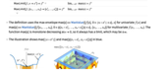
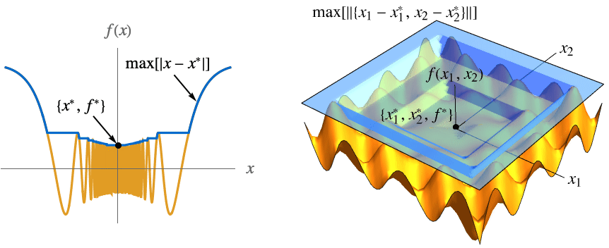
- The definition uses the max envelope max[ϵ]==MaxValue[{f[x],0<
![TemplateBox[{{x, -, {x, ^, *}}}, Abs] TemplateBox[{{x, -, {x, ^, *}}}, Abs]](Files/MaxLimit.en/28.png) <ϵ},x] for univariate f[x] and max[ϵ]==MaxValue[{f[x1,…,xn],0<
<ϵ},x] for univariate f[x] and max[ϵ]==MaxValue[{f[x1,…,xn],0<![TemplateBox[{{{, {{{x, _, {(, 1, )}}, -, {x, _, {(, 1, )}, ^, *}}, ,, ..., ,, {{x, _, n}, -, {x, _, {(, n, )}, ^, *}}}, }}}, Norm] TemplateBox[{{{, {{{x, _, {(, 1, )}}, -, {x, _, {(, 1, )}, ^, *}}, ,, ..., ,, {{x, _, n}, -, {x, _, {(, n, )}, ^, *}}}, }}}, Norm]](Files/MaxLimit.en/29.png) <ϵ},{x1,…,xn}] for multivariate f[x1,…,xn]. The function max[ϵ] is monotone decreasing as ϵ0, so it always has a limit, which may be ±∞.
<ϵ},{x1,…,xn}] for multivariate f[x1,…,xn]. The function max[ϵ] is monotone decreasing as ϵ0, so it always has a limit, which may be ±∞. - The illustration shows max[
![TemplateBox[{{x, -, {x, ^, *}}}, Abs] TemplateBox[{{x, -, {x, ^, *}}}, Abs]](Files/MaxLimit.en/30.png) ] and max[
] and max[ ] in blue.
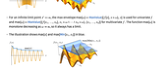
 - For an infinite limit point x*∞, the max envelope max[ω]MaxValue[{f[x],x>ω},x] is used for univariate f and max[ω]MaxValue[{f[x1,…,xn],x1>ω∧⋯∧xn>ω},{x1,…,xn}] for multivariate f. The function max[ω] is monotone decreasing as ω∞, so it always has a limit.
- The illustration shows max[x] and max[Min[x1,x2]] in blue.
- MaxLimit returns unevaluated when the max limit cannot be found.
- The following options can be given:
-
Assumptions $Assumptions assumptions on parameters Direction Reals directions to approach the limit point GenerateConditions Automatic whether to generate conditions on parameters Method Automatic method to use PerformanceGoal "Quality" aspects of performance to optimize - Possible settings for Direction include:
-
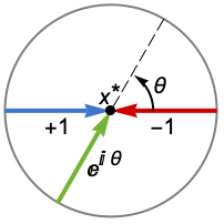
Reals or "TwoSided" from both real directions "FromAbove" or -1 from above or larger values "FromBelow" or +1 from below or smaller values Complexes from all complex directions Exp[ θ] in the direction 
{dir1,…,dirn} use direction diri for variable xi independently - DirectionExp[ θ] at x* indicates the direction tangent of a curve approaching the limit point x*.
- Possible settings for GenerateConditions include:
-
Automatic non-generic conditions only True all conditions False no conditions None return unevaluated if conditions are needed - Possible settings for PerformanceGoal include $PerformanceGoal, "Quality" and "Speed". With the "Quality" setting, MaxLimit typically solves more problems or produces simpler results, but it potentially uses more time and memory.

Examples
open all close allBasic Examples (3)
Scope (35)
Basic Uses (5)
Find the max limit at a point:
Find the max limit at a symbolic point:
Find the max limit at -Infinity:
The nested max limit as ![]() first and then
first and then ![]() :
:
Typeset Limits (4)
Use ![]() Mlim
Mlim![]() to enter the character, and
to enter the character, and ![]() to create an underscript:
to create an underscript:
Take a limit from above or below by using a superscript ![]() or
or ![]() on the limit point:
on the limit point:
After typing zero, use ![]() to create a superscript:
to create a superscript:
To specify a direction of Reals or Complexes, enter the domain as an underscript on the character:
Enter the rule as ![]() ->
->![]() , use
, use ![]() to create an underscript, and type
to create an underscript, and type ![]() reals
reals![]() to enter
to enter ![]() :
:
TraditionalForm formatting:
Elementary Functions (10)
Piecewise Functions (5)
A discontinuous piecewise function:
A left-continuous piecewise function:
The two-sided max limit is the larger of the two:
UnitStep is effectively a right-continuous piecewise function:
RealSign is effectively a discontinuous piecewise function:
Note that ![]() is related to neither value:
is related to neither value:
Find the max limit of Floor as x approaches integer values:
Special Functions (4)
Nested Max Limits (3)
Compute the nested max limit as first ![]() and then
and then ![]() :
:
The same result is obtained by computing two MaxLimit expressions:
Computing the max limit as first ![]() and then
and then ![]() yields a different answer:
yields a different answer:
This is again equivalent to two nested max limits:
The nested max limit as first ![]() and then
and then ![]() is
is ![]() :
:
The nested max limit as first ![]() and then
and then ![]() is
is ![]() :
:
Consider the function for two variables at the origin:
The iterated max limit as ![]() and then
and then ![]() is
is ![]() :
:
The iterated max limit as ![]() and then
and then ![]() is
is ![]() :
:
The true bivariate max limit is ![]() , as points where
, as points where ![]() almost cancels
almost cancels ![]() give arbitrarily large values:
give arbitrarily large values:
For example, this value can be approached along the curve ![]() :
:
Visualize the function and the values along the two axes computed previously:
Multivariate Max Limits (4)
Find the max limit of a multivariate function:
The two nested max limits give different answers:
Approaching the origin along the curve ![]() yields a third result:
yields a third result:
The true two-dimensional max limit of the function is ![]() :
:
This is achieved along the curve ![]() :
:
Visualize the minimum and maximum values near the origin:
Find the max limit of a bivariate function:
The true two-dimensional max limit of the function is ![]() :
:
Note that neither iterated limit gives this result:
Indeed, along any rate ![]() the function is constant:
the function is constant:
The maximum is approached along curves with ![]() close to
close to ![]() , such as
, such as ![]() :
:
Visualize the function and the three max limits computed:
Find the max limit of a bivariate function at the origin:
The true two-dimensional max limit at the origin is ![]() :
:
Re-express the function in terms of polar coordinates:
The polar expression is bounded and disappears as ![]() , leaving the max limit of Sin:
, leaving the max limit of Sin:
Compute the max limit of a trivariate function:
The max limit at the origin is ![]() :
:
Note that the various iterated max limits are 0:
This is because the maximum is achieved along the line ![]() ,
, ![]() :
:
The max limit can also be understood by transforming to spherical coordinates:
Options (10)
Assumptions (1)
Specify conditions on parameters using Assumptions:
Direction (5)
The default direction is Reals:
"TwoSided" is equivalent to Reals:
Max limit in the complex plane:
Compare with the limit over the reals:
Compute the bivariate max limit approach from different quadrants:
Approaching the origin from the first quadrant:
Approaching the origin from the second quadrant:
Approaching the origin from the left half-plane:
GenerateConditions (3)
Return a result without stating conditions:
This result is only valid if n>0:
Return unevaluated if the results depend on the value of parameters:
By default, conditions are generated that return a unique result:
By default, conditions are not generated if only special values invalidate the result:
With GenerateConditions->True, even these non-generic conditions are reported:
PerformanceGoal (1)
Use PerformanceGoal to avoid potentially expensive computations:
The default setting uses all available techniques to try to produce a result:
Applications (13)
Geometry of Max Limits (3)
The function ![]() has a max limit of
has a max limit of ![]() at
at ![]() :
:
This means there must be a sequence ![]() for which
for which ![]() as
as ![]() ; for example,
; for example, ![]() :
:
Numerically, ![]() and
and ![]() quite quickly:
quite quickly:
Compute the two sequence limits exactly:
Note that this sequence limit exists even though ![]() itself does not have a limit as
itself does not have a limit as ![]() :
:
The function ![]() has the limit zero as
has the limit zero as ![]() approaches
approaches ![]() :
:
In increasingly small regions around ![]() ,
, ![]() gets increasingly flat and more of the graph is below
gets increasingly flat and more of the graph is below ![]() :
:
The function ![]() does not have a limit as
does not have a limit as ![]() approaches
approaches ![]() :
:
In increasingly small regions around ![]() ,
, ![]() bounces wildly, but
bounces wildly, but ![]() becomes a better and better ceiling for it:
becomes a better and better ceiling for it:
Asymptotic Analysis (3)
A function ![]() is said to be "big-o of
is said to be "big-o of ![]() " at
" at ![]() , written
, written ![]() , if
, if ![]() :
:
It is possible for functions to share neither relationship:
Thus, ![]() is a reflexive partial order on functions:
is a reflexive partial order on functions:
![]() if
if ![]() goes to zero at least as fast as
goes to zero at least as fast as ![]() :
:
From Taylor's theorem, if ![]() has
has ![]() continuous derivatives around
continuous derivatives around ![]() , then
, then ![]() :
:
This is the fifth-order Taylor polynomial at ![]() :
:
Find the motion of a critically driven mass-spring system:
The motion is oscillatory but becomes arbitrarily large, indicating an instability:
The oscillatory motion is bounded and eventually restricted to ![]() , indicating stability:
, indicating stability:
Continuity (4)
A function is upper semicontinuous at ![]() if
if ![]() . UnitStep is upper semicontinuous at the origin:
. UnitStep is upper semicontinuous at the origin:
On the other hand, RealSign is not upper semicontinuous at the origin:
Consider the following function:
This function is upper semicontinuous at the origin:
This is despite f having neither a left nor a right limit at the origin:
Note that the MaxLimit of f does not depend on the value of f at zero, so any value greater than one would also make f upper semicontinuous:
A function is lower semicontinuous at ![]() if
if ![]() . A real-valued function is continuous iff it is both upper and lower semicontinuous. SawtoothWave is lower semicontinuous at
. A real-valued function is continuous iff it is both upper and lower semicontinuous. SawtoothWave is lower semicontinuous at ![]() :
:
However, it is not upper semicontinuous, so it is discontinuous at the origin:
On the other hand, the following shows that TriangleWave is continuous at the origin:
Floor is discontinuous but upper semicontinuous at every integer:
On the other hand, Ceiling is neither continuous nor upper semicontinuous at the integers:
Both are continuous at noninteger values, but only Floor is upper semicontinuous on all of ![]() :
:
Differentiation (3)
The left-upper Dini derivative ![]() is defined as:
is defined as:
The right-upper Dini derivative ![]() is defined similarly:
is defined similarly:
Ramp has finite upper Dini derivatives on the whole real line:
Note that these two derivatives are equal everywhere except the origin:
This is a reflection of the fact that Ramp is differentiable everywhere except the origin:
Consider the following function:
It is continuous at the origin:
But it has neither a left nor a right derivative:
It does, however, have finite Dini derivatives:
This indicates that the growth of the function around zero is bounded:
There are two right Dini derivatives. The first is the right-upper Dini derivative ![]() , defined as follows:
, defined as follows:
The right-lower Dini derivative ![]() is defined similarly using a min limit:
is defined similarly using a min limit:
![]() is right differentiable at
is right differentiable at ![]() if and only if the two are equal and finite, as in the case of Ramp at
if and only if the two are equal and finite, as in the case of Ramp at ![]() :
:
However, the function ![]() does not have a right derivative at the origin:
does not have a right derivative at the origin:
Properties & Relations (13)
A real-valued function always has a (possibly infinite) max limit:
The corresponding limit does not exist:
Positive multiplicative constants can be moved outside a max limit:
If ![]() and
and ![]() have finite max limits as
have finite max limits as ![]() , then
, then ![]() :
:
In this case, there is strict inequality:
Assumptions apply to parameters in the max limit expression:
Direction places conditions on the limit variable:
When computing nested max limits, appropriate assumptions are generated on later limit variables:
For a real-valued function, if Limit exists, then MaxLimit has the same value:
If ![]() has a finite limit as
has a finite limit as ![]() , then
, then ![]() :
:
MaxLimit is always greater than or equal to MinLimit:
If MaxLimit and MinLimit are equal, then the limit exists and equals their common value:
If the max limit is ![]() , then the min limit and thus the limit are also
, then the min limit and thus the limit are also ![]() :
:
MaxLimit can be computed as -MinLimit[-f,…]:
If the two max limits are equal—as in this example—then ![]() has a limit as
has a limit as ![]() :
:
This is a generalization of the "squeezing" or "sandwich" theorem:
MaxLimit is always greater than or equal to DiscreteMaxLimit:
Possible Issues (1)
MaxLimit is only defined for real-valued functions:
Related Guides
History
Text
Wolfram Research (2017), MaxLimit, Wolfram Language function, https://reference.wolfram.com/language/ref/MaxLimit.html.
CMS
Wolfram Language. 2017. "MaxLimit." Wolfram Language & System Documentation Center. Wolfram Research. https://reference.wolfram.com/language/ref/MaxLimit.html.
APA
Wolfram Language. (2017). MaxLimit. Wolfram Language & System Documentation Center. Retrieved from https://reference.wolfram.com/language/ref/MaxLimit.html
BibTeX
@misc{reference.wolfram_2025_maxlimit, author="Wolfram Research", title="{MaxLimit}", year="2017", howpublished="\url{https://reference.wolfram.com/language/ref/MaxLimit.html}", note=[Accessed: 29-March-2026]}
BibLaTeX
@online{reference.wolfram_2025_maxlimit, organization={Wolfram Research}, title={MaxLimit}, year={2017}, url={https://reference.wolfram.com/language/ref/MaxLimit.html}, note=[Accessed: 29-March-2026]}