"KernelDensityEstimation" (机器学习方法)
"KernelDensityEstimation" (机器学习方法)
- LearnDistribution 的方法.
- 模拟带有混合简单分布的概率密度.
Details & Suboptions
- "KernelDensityEstimation" 是一种非参数方法,它使用以每个训练示例为中心的简单分布(称为内核)的混合来模拟数值空间的概率密度,如在 KernelMixtureDistribution 中的一样.
- 向量
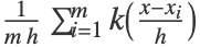
 的概率密度函数为:
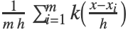 ,其中,内核函数
 、内核大小
 以及培训范例数 m.
- 可以给出以下选项:
-
Method "Fixed" 内核大小方法 "KernelSize" Automatic 当 Method"Fixed" 时的内核大小 "KernelType" "Gaussian" 使用的内核类型 "NeighborsNumber" Automatic 表示为邻域数的内核大小 - "KernelType" 的可能设置包括:
-
"Gaussian" 每个内核是一个高斯分布 "Ball" 每个内核是球中的均匀分布 - Method 的可能设置包括:
-
"Adaptive" 内核大小彼此不同 "Fixed" 所有内核有同样的大小 - 当 "KernelType""Gaussian",每个内核是个球形高斯(独立正态分布
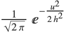 的乘积),并且 "KernelSize" h 指的是正态分布的标准偏差.
- 当 "KernelType""Ball",每个内核是球内的均匀分布,并且 "KernelSize" 指的是球的半径.
- "NeighborsNumber"k 的值被转换成内核大小,因此,以培训范例为中心的内核一般 "包含" k 个其他培训范例. 如果 "KernelType""Ball","包含" 指的是球内的范例. 如果 "KernelType""Gaussian","包含" 指的是半径为 h
 的球内的范例,其中,n 是数据的维数.
- 当 Method"Fixed" 并且 "NeighborsNumber"k,则找到唯一的内核大小,例如,培训范例包含平均 k 个其他范例.
- 当 Method"Adaptive" 并且 "NeighborsNumber"k, 每个培训范例自适应其内核大小,例如包含大概 k 个其他范例.
- 因为预处理,"NeighborsNumber" 选项一般比 "KernelSize" 更方便控制内核大小. 当 Method"Fixed","KernelSize" 值取代 "NeighborsNumber" 值.
- Information[LearnedDistribution[…],"MethodOption"] 可用于提取由自动系统选择的选项值.
- LearnDistribution[…,FeatureExtractor"Minimal"] 可用于删除大部分预处理和直接访问的方法.
范例
打开所有单元 关闭所有单元基本范例 (3)
在数值数据集上培训 "KernelDensityEstimation" 分布:
ld = LearnDistribution[{1.2, 2.1, 3.5, 4.3}, Method -> "KernelDensityEstimation"]查询分布 Information:
Information[ld]Information[ld, "MethodOption"]Information[ld, "KernelType"]PDF[ld, 1.3]Show[Plot[PDF[ld, x], {x, -6, 12}, Filling -> Bottom], NumberLinePlot[{1.2, 2.1, 3.5, 4.3}, Spacings -> 0, PlotStyle -> Red]]Histogram[RandomVariate[ld, 10000], 50]在二维数据集上培训 "KernelDensityEstimation" 分布:
iris = ExampleData[{"MachineLearning", "FisherIris"}, "Data"][[All, 1, {1, 3}]];ld = LearnDistribution[iris, Method -> "KernelDensityEstimation"]Show[ContourPlot[PDF[ld, {x, y}], {x, 4, 8}, {y, 1, 7}, PlotRange -> All, Contours -> 10], ListPlot[iris, PlotStyle -> Red]]使用 SynthesizeMissingValues 估算使用学习分布的丢失值:
SynthesizeMissingValues[ld, {5.5, Missing[]}]Histogram[Table[Last@SynthesizeMissingValues[ld, {5.5, Missing[]}], 1000]]在标称数据集上,培训 "KernelDensityEstimation" 分布:
ld = LearnDistribution[{"A", "A", "B", "B", "B"}, Method -> "KernelDensityEstimation"]PDF[ld, "A"]PDF[ld, "A"]使用 ComputeUncertainty 获取结果中的不确定性:
PDF[ld, "A", ComputeUncertainty -> True]增加 MaxIterations 提高估计精度:
PDF[ld, "A", MaxIterations -> 1000, ComputeUncertainty -> True]选项 (4)
"KernelSize" (1)
iris = ExampleData[{"MachineLearning", "FisherIris"}, "Data"][[All, 1, {1, 3}]];ld = LearnDistribution[iris, Method -> {"KernelDensityEstimation", "KernelSize" -> 0.2}]PDF[ld, {6, 4}]plots = (
ld = LearnDistribution[iris, Method -> {"KernelDensityEstimation", "KernelSize" -> #}, FeatureExtractor -> "Minimal"];
Show[ContourPlot[PDF[ld, {x, y}], {x, 2, 10}, {y, 0, 8}, PlotRange -> All, Contours -> 10], ListPlot[iris, PlotStyle -> Red], ImageSize -> 250, PlotLabel -> "h = " <> ToString[#]]
) & /@ {0.05, 0.1, 0.2, 0.35, 0.5, 1};Grid[Partition[plots, 2]]"KernelType" (1)
用 "Ball" 内核培训 "KernelDensityEstimation" 分布:
iris = ExampleData[{"MachineLearning", "FisherIris"}, "Data"][[All, 1, {1, 3}]];ld = LearnDistribution[iris, Method -> {"KernelDensityEstimation", "KernelType" -> "Ball"}]PDF[ld, {6, 4}]可视化用 "Ball" 和 "Gaussian" 内核培训内核混合分布后获得的 PDF:
plots = (ld = LearnDistribution[iris, Method -> {"KernelDensityEstimation", "KernelType" -> #}, FeatureExtractor -> "Minimal"];
Show[ContourPlot[PDF[ld, {x, y}], {x, 2, 10}, {y, 0, 8}, PlotRange -> All, Contours -> 10, PlotLabel -> #], ListPlot[iris, PlotStyle -> Red], ImageSize -> 250]) & /@ {"Ball", "Gaussian"};Row[plots]Method (1)
培训带有 "Adaptive" 方法的 "KernelDensityEstimation" 分布:
iris = ExampleData[{"MachineLearning", "FisherIris"}, "Data"][[All, 1, {1, 3}]];ld = LearnDistribution[iris, Method -> {"KernelDensityEstimation", Method -> "Adaptive"}]PDF[ld, {6, 4}]可视化用 "Ball" 和 "Gaussian" 内核培训内核混合分布后获得的 PDF:
plots = (ld = LearnDistribution[iris, Method -> {"KernelDensityEstimation", Method -> #}, FeatureExtractor -> "Minimal"];
Show[ContourPlot[PDF[ld, {x, y}], {x, 2, 10}, {y, 0, 8}, PlotRange -> All, Contours -> 10, PlotLabel -> #], ListPlot[iris, PlotStyle -> Red], ImageSize -> 250]) & /@ {"Fixed", "Adaptive"};Row[plots]"NeighborsNumber" (1)
iris = ExampleData[{"MachineLearning", "FisherIris"}, "Data"][[All, 1, {1, 3}]];ld = LearnDistribution[iris, Method -> {"KernelDensityEstimation", "NeighborsNumber" -> 10}]PDF[ld, {6, 4}]可视化培训带有各种内核大小(表示为邻域数)的内核混合分布后获得的 PDF:
plots = (
	ld = LearnDistribution[iris, Method -> {"KernelDensityEstimation", "NeighborsNumber" -> #}, FeatureExtractor -> "Minimal"];
	Show[ContourPlot[PDF[ld, {x, y}], {x, 2, 10}, {y, 0, 8}, PlotRange -> All, Contours -> 10], ListPlot[iris, PlotStyle -> Red], ImageSize -> 250, PlotLabel -> "k = " <> ToString[#]]
) & /@ {1, 2, 5, 10, 20, 50};Grid[Partition[plots, 2]]
 《Wolfram 语言入门》:机器学习