Library Dependency

This is a placeholder model. It requires the PlanarMechanics library.

• The free PlanarMechanics library was created especially for modeling multibody systems with two-dimensional mechanical components. Compared to the MultiBody library, currently available in the Modelica Standard Library, it is simpler to use and it is more optimized to planar modeling. Planar models of mechanical systems are useful in many different applications, for example, in contact problems that are more easily modeled in 2D than in 3D.

The following documentation is taken from the main example of the downloadable model. Once you have downloaded all the model dependencies, the model can be downloaded here.

Wheel with Dry Friction

Introduction

Although wheeled vehicles have been an important mode of transportation for more than 5,000 years, the dynamic behavior of wheel-surface interactions is still quite tricky to understand. Here, we study how a wheel modeled with dry friction behaves when driven with a constant torque around a pole. The Planar Mechanics Library and Modelica Standard Library have been used to create this model.

Simulation

To simulate the model and see the generated 3D animation, follow the steps below:

• Click the Simulate button .
• When the simulation is finished, click the Animate button in Simulation Center.
• Use your mouse or trackpad to drag the animation into a good angle and zoom in with your scroll wheel or by using the trackpad. Then click the Play button to play the animation.

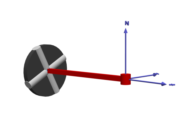
Above is an automatically generated 3D visualization of the model. To the left is the revolute joint fixed at a point in space. Attached to the revolute joint is a prismatic joint that leads to the wheel.

Analysis

When you have simulated the model, a stored plot will automatically be displayed, showing a parametric plot over the wheel position. Click on the other stored plot to see slip and adhesion velocities.

The first stored plot looks like this:

In the parametric plot above, we can see the position of the wheel in a two-dimensional plane. As the wheel starts accelerating, the distance from the center will increase due to lateral slipping. Initially, this slipping is small, and the wheel moves in an almost ideal circle. However, as the slip velocity increases as a result of an increasing centrifugal force, the wheel starts to slide.

The second stored plot looks like this:

In the plot above, the slip velocity has been plotted against time to see when and how fast the wheel slipped.

The sliding of the wheel can be understood by studying the force of friction on the wheel as a function of slip velocity. See the CDF document for more examples of plots to study this phenomenon further.

Plotting and Further Analysis

To further investigate this system, try changing some parameters in the model and see what happens. Interesting parameters to change are, for example, torque applied to the wheel, wheel radius, friction coefficients at adhesion or sliding, and so on. Investigate the result by plotting the plots above again but with other parameter values. Other interesting quantities are, for example, friction force versus slip velocity, or centrifugal force and friction force versus time.

• To create a new plot, click the toolbar icon .
• To plot a variable, check its checkbox in the Plot window on the left in Simulation Center.
• To create a new subplot, click the toolbar icon .
• To plot two variables against each other in a parametric plot, click the toolbar icon and check the checkboxes of the two variables to plot.
• To change a parameter value, first click Parameters next to the Plot tab.
• Change a parameter by opening up a tree in the Parameters view and changing the value for the parameter you want to change. Then run the simulation again.

Terms and Conditions of Use