TsallisQGaussianDistribution[μ,β,q]
represents a Tsallis ![]() -Gaussian distribution with mean μ, scale parameter β, and deformation parameter q.
-Gaussian distribution with mean μ, scale parameter β, and deformation parameter q.
TsallisQGaussianDistribution[q]
represents a Tsallis ![]() -Gaussian distribution with mean 0 and scale parameter 1.
-Gaussian distribution with mean 0 and scale parameter 1.


TsallisQGaussianDistribution
TsallisQGaussianDistribution[μ,β,q]
represents a Tsallis ![]() -Gaussian distribution with mean μ, scale parameter β, and deformation parameter q.
-Gaussian distribution with mean μ, scale parameter β, and deformation parameter q.
TsallisQGaussianDistribution[q]
represents a Tsallis ![]() -Gaussian distribution with mean 0 and scale parameter 1.
-Gaussian distribution with mean 0 and scale parameter 1.
Details
- TsallisQGaussianDistribution allows μ to be any real number, β to be any positive real number, and q to be any real number less than 3.
- TsallisQGaussianDistribution allows μ and β to be any quantities of the same unit dimensions, and λ to be a dimensionless quantity. »
- TsallisQGaussianDistribution can be used with such functions as Mean, CDF, and RandomVariate.
Background & Context
- TsallisQGaussianDistribution[μ,β,q] represents a continuous statistical distribution parametrized by a positive real number β (called a "scale parameter") and by real numbers μ and
 (the mean of the distribution and a "deformation parameter", respectively), which together determine the overall behavior of its probability density function (PDF). In general, the PDF of a Tsallis
  -Gaussian distribution is unimodal with a single "peak" (i.e. a global maximum), though its overall shape (its support, its height, its spread, and the horizontal location of its maximum) is determined by the values of μ, β, and
  . In addition, the tails of the PDF (which are defined only when
  ) are typically "fat" (i.e. the PDF decreases non-exponentially for large values
  ) but are "thin" (i.e. the PDF decreases exponentially for large
  ) for
) for  . (When defined, this behavior can be made quantitatively precise by analyzing the SurvivalFunction of the distribution.) The Tsallis
  -Gaussian distribution is often referred to merely as the
  -Gaussian distribution, while the one-parameter form TsallisQGaussianDistribution[q] is equivalent to TsallisQGaussianDistribution[0,1,q] and is sometimes referred to as the standard
  -Gaussian distribution.
 - The Tsallis
 -Gaussian distribution is named for Brazilian physicist Constantino Tsallis and is derived via maximization of the so-called Tsallis entropy (in statistical mechanics) subject to certain conditions. Along with the related
  -exponential distribution, the
  -Gaussian distribution is one of a family of probability distributions referred to collectively as Tsallis distributions and derived according to the above-mentioned process. The
  -Gaussian distribution has also been used to model phenomena like wealth distribution and asset pricing in fields such as economics, finance, and actuarial science.
 - RandomVariate can be used to give one or more machine- or arbitrary-precision (the latter via the WorkingPrecision option) pseudorandom variates from a
 -Gaussian distribution. Distributed[x,TsallisQGaussianDistribution[μ,β,q]], written more concisely as xTsallisQGaussianDistribution[μ,β,q], can be used to assert that a random variable x is distributed according to a
  -Gaussian distribution. Such an assertion can then be used in functions such as Probability, NProbability, Expectation, and NExpectation.
 - The probability density and cumulative distribution functions for
 -Gaussian distributions may be given using PDF[TsallisQGaussianDistribution[μ,β,q],x] and CDF[TsallisQGaussianDistribution[μ,β,q],x]. The mean, median, variance, raw moments, and central moments may be computed using Mean, Median, Variance, Moment, and CentralMoment, respectively.
 - DistributionFitTest can be used to test if a given dataset is consistent with a
 -Gaussian distribution, EstimatedDistribution to estimate a parametric
  -Gaussian distribution from given data, and FindDistributionParameters to fit data to a
  -Gaussian distribution. ProbabilityPlot can be used to generate a plot of the CDF of given data against the CDF of a symbolic
  -Gaussian distribution, and QuantilePlot to generate a plot of the quantiles of given data against the quantiles of a symbolic
  -Gaussian distribution.
 - TransformedDistribution can be used to represent a transformed
 -Gaussian distribution, CensoredDistribution to represent the distribution of values censored between upper and lower values, and TruncatedDistribution to represent the distribution of values truncated between upper and lower values. CopulaDistribution can be used to build higher-dimensional distributions that contain a
  -Gaussian distribution, and ProductDistribution can be used to compute a joint distribution with independent component distributions involving
  -Gaussian distributions.
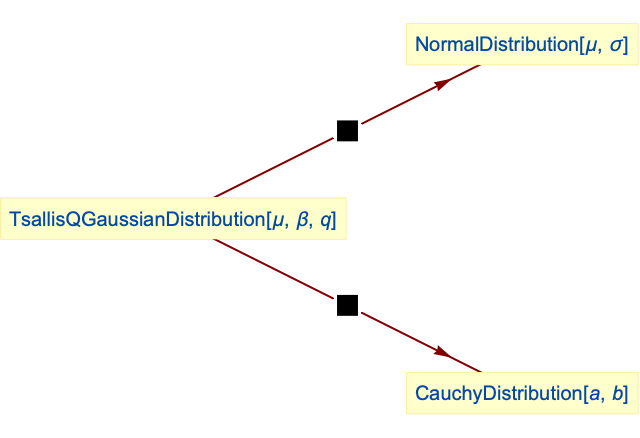
 - TsallisQGaussianDistribution is related to a number of other distributions. TsallisQGaussianDistribution is an immediate generalization of NormalDistribution, in the sense that the PDF of TsallisQGaussianDistribution[μ,β,1] is precisely the same as that of NormalDistribution[μ,β] (for
 ). TsallisQGaussianDistribution can be realized as an instance of CauchyDistribution, in that TsallisQGaussianDistribution[μ,β,2] is equivalent to CauchyDistribution[μ,β
  ] and is also closely related to TsallisQExponentialDistribution, ExponentialDistribution, StudentTDistribution, and WeibullDistribution.
Examples
open all close allBasic Examples (4)
Scope (8)
Generate a sample of pseudorandom numbers from a ![]() -Gaussian distribution:
-Gaussian distribution:
Compare the histogram to the PDF:
Distribution parameters estimation:
Estimate the distribution parameters from sample data:
Compare the density histogram of the sample with the PDF of the estimated distribution:
Different moments with closed forms as functions of parameters:
Closed form for symbolic order:
Hazard function for some fixed q values:
Quantiles can be evaluated in closed form for certain rational values of q:
Consistent use of Quantity in parameters yields QuantityDistribution:
Applications (1)
The ![]() -Gaussian distribution can be used to model differences in log returns of stock prices:
-Gaussian distribution can be used to model differences in log returns of stock prices:
Fit the distribution to the data and compare to the fit with NormalDistribution:
Compare the histogram of the data to the PDF:
Inspect the heavy-tail behavior:
Find the probability that the log-difference in price is above $0.1:
Simulate the log-difference in price for 30 consecutive days:
Properties & Relations (5)
The ![]() -Gaussian distribution is closed under scaling and translation:
-Gaussian distribution is closed under scaling and translation:
For q that is close to 1, TsallisQGaussianDistribution resembles NormalDistribution:
Relationships to other distributions:
The ![]() -Gaussian distribution simplifies to NormalDistribution for
-Gaussian distribution simplifies to NormalDistribution for ![]() :
:
The ![]() -Gaussian distribution simplifies to CauchyDistribution for
-Gaussian distribution simplifies to CauchyDistribution for ![]() :
:
Possible Issues (2)
TsallisQGaussianDistribution is not defined when μ is not a real number:
TsallisQGaussianDistribution is not defined when β is not a positive real number:
TsallisQGaussianDistribution is not defined when q is not a real number less than 3:
Substitution of invalid parameters into symbolic outputs gives results that are not meaningful:
Text
Wolfram Research (2012), TsallisQGaussianDistribution, Wolfram Language function, https://reference.wolfram.com/language/ref/TsallisQGaussianDistribution.html (updated 2016).
CMS
Wolfram Language. 2012. "TsallisQGaussianDistribution." Wolfram Language & System Documentation Center. Wolfram Research. Last Modified 2016. https://reference.wolfram.com/language/ref/TsallisQGaussianDistribution.html.
APA
Wolfram Language. (2012). TsallisQGaussianDistribution. Wolfram Language & System Documentation Center. Retrieved from https://reference.wolfram.com/language/ref/TsallisQGaussianDistribution.html