StableDistribution

StableDistribution[type,α,β,μ,σ]

represents the stable distribution S_type with index of stability α, skewness parameter β, location parameter μ, and scale parameter σ.

Details

A linear combination of independent identically distributed stable random variables is also stable.
A stable distribution is defined in terms of its characteristic function , which satisfies a functional equation where for any and there exist and such that . The general solution to the functional equation has four parameters.
StableDistribution allows 0<α≤2, -1≤β≤1, μ to be any real number, and σ to be any positive real number.
StableDistribution allows μ and σ to be any quantities of the same unit dimensions, and α, β to be dimensionless quantities. »
CharacteristicFunction[StableDistribution[0,α,…],t] is continuous in α and given by $exp(i mu t-sigma TemplateBox[{t}, Abs] (1+2i beta/pi sgn(t) log(TemplateBox[{{t, , sigma}}, Abs]))) alpha=1; exp(i mu t-TemplateBox[{{t, , sigma}}, Abs]^alpha (1+i beta tan((pi alpha)/2) sgn(t) (TemplateBox[{{t, , sigma}}, Abs]^(1-alpha)-1))) alpha!=1$ .
CharacteristicFunction[StableDistribution[1,α,…],t] is discontinuous in α and given by $exp(i mu t-sigma TemplateBox[{t}, Abs] (1+2 i beta/pi sgn(t) log(TemplateBox[{t}, Abs]))) alpha=1; exp(i mu t-TemplateBox[{{t, , sigma}}, Abs]^alpha (1-i beta tan((pi alpha)/2) sgn(t))) alpha!=1$ .
StableDistribution[α] is equivalent to StableDistribution[1,α,0,0,1].
StableDistribution[α,β] is equivalent to StableDistribution[1,α,β,0,1].
StableDistribution[α,β,μ,σ] is equivalent to StableDistribution[1,α,β,μ,σ].
StableDistribution can be used with such functions as Mean, CDF, and RandomVariate.

Background & Context

StableDistribution[type,α,β,μ,σ] represents a continuous statistical distribution belonging to one of two types and parametrized by the positive real number σ (called a "scale parameter") and by the real numbers μ (a "location parameter"), α (the index of stability of the distribution for which ), and β (a "skewness parameter" satisfying ), which together determine the overall behavior of its probability density function (PDF).
In general, the PDF of a stable distribution is unimodal with a single "peak" (i.e. a global maximum), though its overall shape (its height, its spread, and the horizontal location of its maximum) is determined both by its type and by the values of α, β, μ, and σ. In addition, the tails of the PDF may be "fat" (i.e. the PDF decreases non-exponentially for large values ) or "thin" (i.e. the PDF decreases exponentially for large ), depending on the values of type, α, β, μ, and σ. (This behavior can be made quantitatively precise by analyzing the SurvivalFunction of the distribution.) The four-, two-, and one-parameter versions StableDistribution[α,β,μ,σ], StableDistribution[α,β], and StableDistribution[α] are equivalent to the type-1 distributions StableDistribution[1,α,β,μ,σ], StableDistribution[1,α,β,0,1], and StableDistribution[1,α,0,0,1], respectively. For various values of its parameters, the stable distribution may be referred to as the stable-Paretian distribution, the Pareto–Lévy distribution (not to be confused with ParetoDistribution or LevyDistribution), or as the Lévy α-stable distribution. The stable distribution is also distinct from the similarly named min- and max-stable distributions (MinStableDistribution and MaxStableDistribution, respectively).
Despite many special cases of the stable distribution being classical in nature, the family of stable distributions described above was first studied by mathematician Paul Lévy in the mid-1920s. The family of stable distributions is characterized by being closed under linear combinations, meaning their PDFs in general do not have closed-form expression and must instead be described in terms of their characteristic functions (CharacteristicFunction). Stable distributions are particularly important in stochastics and probability due to the role they play in generalizing the so-called central limit theorem, though such distributions have also been used to model phenomena in finance, astronomy, and physics.
RandomVariate can be used to give one or more machine- or arbitrary-precision (the latter via the WorkingPrecision option) pseudorandom variates from a stable distribution. Distributed[x,StableDistribution[type,α,β,μ,σ]], written more concisely as xStableDistribution[type,α,β,μ,σ], can be used to assert that a random variable x is distributed according to a stable distribution of a given type. Such an assertion can then be used in functions such as Probability, NProbability, Expectation, and NExpectation.
The probability density and cumulative distribution functions for stable distributions of a given type may be given using PDF[StableDistribution[type,α,β,μ,σ],x] and CDF[StableDistribution[type,α,β,μ,σ],x]. The mean, median, variance, raw moments, and central moments may be computed using Mean, Median, Variance, Moment, and CentralMoment, respectively.
DistributionFitTest can be used to test if a given dataset is consistent with a stable distribution, EstimatedDistribution to estimate a stable parametric distribution from given data, and FindDistributionParameters to fit data to a stable distribution. ProbabilityPlot can be used to generate a plot of the CDF of given data against the CDF of a symbolic stable distribution, and QuantilePlot to generate a plot of the quantiles of given data against the quantiles of a symbolic stable distribution.
TransformedDistribution can be used to represent a transformed stable distribution, CensoredDistribution to represent the distribution of values censored between upper and lower values, and TruncatedDistribution to represent the distribution of values truncated between upper and lower values. CopulaDistribution can be used to build higher-dimensional distributions that contain a stable distribution, and ProductDistribution can be used to compute a joint distribution with independent component distributions involving stable distributions.
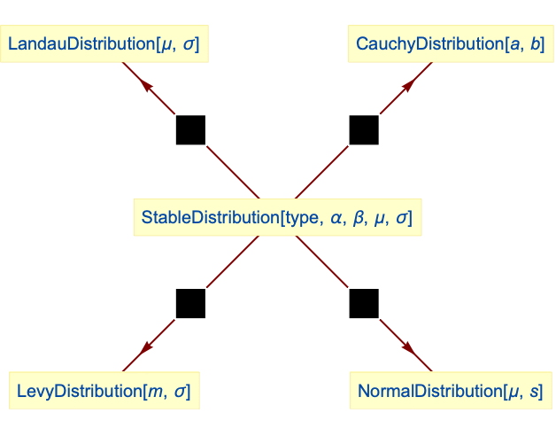
StableDistribution is closely related to a number of other distributions. LandauDistribution, CauchyDistribution, NormalDistribution, and LevyDistribution are examples of type-1 stable distributions in the sense that LandauDistribution[μ,σ] has the same characteristic function (CharacteristicFunction) as StableDistribution[1,1,1,μ,σ], CauchyDistribution[0,1] has the same PDF as StableDistribution[1,1,0,0,1], the PDF of NormalDistribution[μ,σ] is equivalent to that of StableDistribution[1,2,β,μ,σ/], and the PDF of LevyDistribution[μ,σ] is precisely the same as that of StableDistribution[1,1/2,1,μ,σ]. Qualitatively, StableDistribution is similar to PearsonDistribution, and it is also closely related to ParetoDistribution, BetaDistribution, GammaDistribution, and HalfNormalDistribution.

Examples

open allclose all

Basic Examples (4)

Probability density function for type 1 for a range of skewness parameters:

Probability density function for type 0 for various stability indexes:

Cumulative distribution function for type 1:

Type 0:

Mean depends on the type:

Variance is type independent and is only defined for :

Scope (4)

Generate a sample of pseudorandom numbers from a stable distribution:

Compare its histogram to the PDF:

Higher moments are only defined for :

This is the case where StableDistribution reduces to NormalDistribution:

Hazard function for different stability indexes:

Hazard function for different skewness parameters:

Consistent use of Quantity in parameters yields QuantityDistribution:

Find the 75% quantile:

Applications (9)

Assuming daily logarithmic return of the stock market follows a stable distribution, simulate and visualize stock prices over a period of 5 years:

Assuming stock logarithmic return follows a stable distribution, find the value at risk at the 95% level:

Compute the 95% value at risk point loss of the current S&P 500 index value, assuming the above distribution:

Find the expected shortfall of logarithmic return:

Compute the associated point loss:

Fit the daily logarithm return of the IBM stocks since January 1, 2005 to a stable distribution:

Compute logarithmic returns:

Fit logarithmic returns to a stable distribution:

Compare the estimated distribution to a data histogram:

The product of a symmetric stable random variate and the power of an exponential random variate follows a Linnik distribution:

Calculate the characteristic function of a Linnik distribution:

Generate random variates and show the histogram:

Map–Airy distribution [MathWorld] is a member of the stable family:

Its probability density is known in closed form:

Find the location of the mode:

Estimate the parameter of stable distribution from a sample characteristic function:

Plot absolute values of a sample characteristic function and a population characteristic function:

Compare with the maximum likelihood estimation:

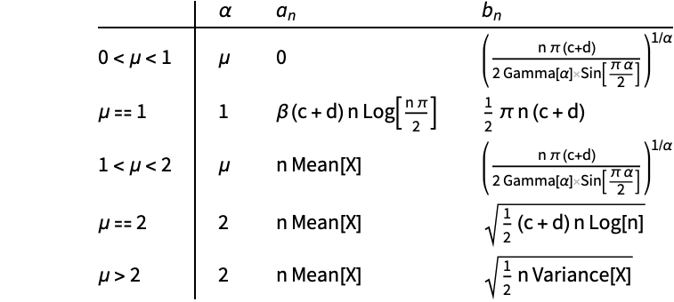
Generalized central limit theorem gives sequences and such that the distribution of the shifted and rescaled sum of i.i.d. random variates whose distribution function has asymptotes as and as weakly converges to the stable distribution :

Illustrate the generalized central limit theorem using a two-sided Pareto distribution:

Define the mean and variance of the two-sided Pareto distribution for future use:

Define a routine to generate -variates:

Define a function to visualize a density plot and data histogram:

Case of :

Case of standard central limit theorem, i.e. :

Holtsmark distribution is the distribution of forces acting on a particle in an infinite Poisson system. The ‐component of the gravitational force follows symmetric stable distribution: