Algebraic Manipulation
Algebraic Manipulation
| Expand[poly] | expand out products and powers |
| Factor[poly] | factor completely |
| FactorTerms[poly] | pull out any overall numerical factor |
| FactorTerms[poly,{x,y,…}] | pull out any overall factor that does not depend on x, y, … |
| Collect[poly,x] | arrange a polynomial as a sum of powers of x |
| Collect[poly,{x,y,…}] | arrange a polynomial as a sum of powers of x, y, … |
Expand expands out products and powers, writing the polynomial as a simple sum of terms:
Factor performs complete factoring of the polynomial:
There are several ways to write any polynomial. The functions Expand, FactorTerms, and Factor give three common ways. Expand writes a polynomial as a simple sum of terms, with all products expanded out. FactorTerms pulls out common factors from each term. Factor does complete factoring, writing the polynomial as a product of terms, each of as low degree as possible.
When you have a polynomial in more than one variable, you can put the polynomial in different forms by essentially choosing different variables to be "dominant". Collect[poly,x] takes a polynomial in several variables and rewrites it as a sum of terms containing different powers of the "dominant variable" x.
If you specify a list of variables, Collect will effectively write the expression as a polynomial in these variables:
| Expand[poly,patt] | expand out poly, avoiding those parts which do not contain terms matching patt |
| PowerExpand[expr] | expand out (ab)c and (ab)c in expr |
| PowerExpand[expr,Assumptions->assum] | |
expand out expr assuming assum | |
The Wolfram System does not automatically expand out expressions of the form (ab)c except when c is an integer. In general it is only correct to do this expansion if a and b are positive reals. Nevertheless, the function PowerExpand does the expansion, effectively assuming that a and b are indeed positive reals.
Log is not automatically expanded out:
PowerExpand does the expansion:
PowerExpand returns a result correct for the given assumptions:
| Collect[poly,patt] | collect separately terms involving each object that matches patt |
| Collect[poly,patt,h] | apply h to each final coefficient obtained |
This applies Factor to each coefficient obtained:
| HornerForm[expr,x] | puts expr into Horner form with respect to x |
Horner form is a way of arranging a polynomial that allows numerical values to be computed more efficiently by minimizing the number of multiplications.
| PolynomialQ[expr,x] | test whether expr is a polynomial in x |
| PolynomialQ[expr,{x1,x2,…}] | test whether expr is a polynomial in the xi |
| Variables[poly] | a list of the variables in poly |
| Exponent[poly,x] | the maximum exponent with which x appears in poly |
| Coefficient[poly,expr] | the coefficient of expr in poly |
| Coefficient[poly,expr,n] | the coefficient of exprn in poly |
| Coefficient[poly,expr,0] | the term in poly independent of expr |
| CoefficientList[poly,{x1,x2,…}] | generate an array of the coefficients of the xi in poly |
| CoefficientRules[poly,{x1,x2,…}] | get exponent vectors and coefficients of monomials |
This gives the maximum exponent with which x appears in the polynomial t. For a polynomial in one variable, Exponent gives the degree of the polynomial:
Coefficient[poly,expr] gives the total coefficient with which expr appears in poly. In this case, the result is a sum of two terms:
This is equivalent to Coefficient[t,x^2]:
For multivariate polynomials, CoefficientList gives an array of the coefficients for each power of each variable:
CoefficientRules includes only those monomials that have nonzero coefficients:
It is important to notice that the functions in this tutorial will often work even on polynomials that are not explicitly given in expanded form.
Without giving specific integer values to a, b, and c, this expression cannot strictly be considered a polynomial:
Exponent[expr,x] still gives the maximum exponent of x in expr, but here has to write the result in symbolic form:
The leading term of a polynomial can be chosen in many different ways. For multivariate polynomials, sorting by the total degree of the monomials is often useful.
| MonomialList[poly] | get the list of monomials |
| CoefficientRules[poly] | represent the monomials by exponent vectors and coefficients |
| FromCoefficientRules[list] | construct a polynomial from a list of rules |
FromCoefficientRules constructs the original polynomial from the list of rules and variables:
If the second argument to MonomialList or CoefficientRules is omitted, the variables are taken in the order in which they are returned by the function Variables.
By default, the monomials are sorted lexicographically and given in the decreasing order. In the previous example, {5,4,1} (corresponding to  ) is taken to precede {5,3,2} (corresponding to
  ) by the second element.
An order is described by defining how two vectors of exponents  and
and  are sorted. For the lexicographic order,
An order can also be described by giving a weight matrix. In that case the exponent vectors are multiplied by the weight matrix and the results are sorted lexicographically, also in the decreasing order. The matrices for different orderings are given as follows.

For functions such as GroebnerBasis and PolynomialReduce, it is necessary that the order be well-founded, which ensures that any decreasing sequence of elements is finite (the elements being the vectors of non-negative exponents). In order for that condition to hold, the first nonzero value in each column of the weight matrix must be positive.
The default sorting used for polynomial terms in an expression corresponds to the negative lexicographic ordering with variables sorted in the reversed order. This is commonly known as reverse lexicographic ordering.
This is the internal representation of a polynomial. The arguments of Plus and Times are sorted on evaluation:
TraditionalForm tries to arrange the terms in an order close to the lexicographic ordering.
The polynomial displayed in TraditionalForm:
This uses advanced typesetting capabilities to obtain the list of terms in the same order as they appear in the TraditionalForm output:
The option ParameterVariables tells TraditionalForm which variables should be excluded from the ordering.
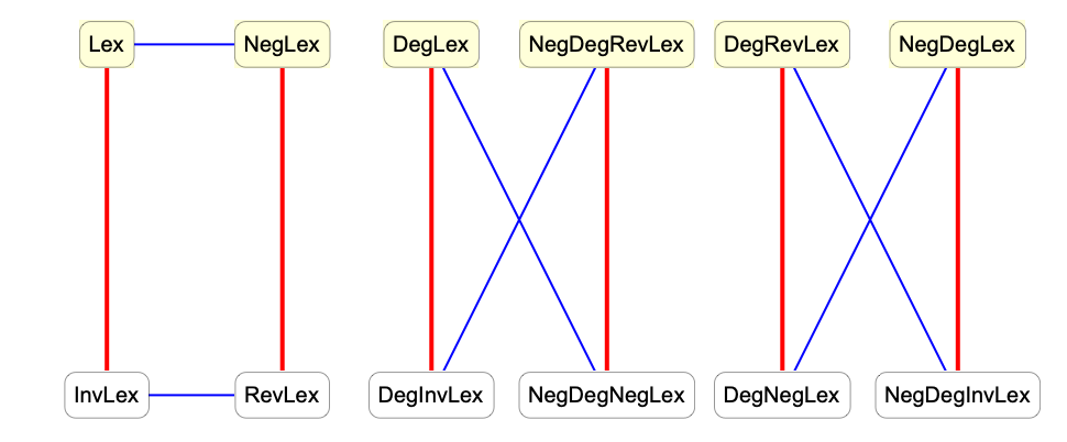
One can obtain additional orderings from the six orderings used in MonomialList simply by reversing the resulting list. This is effectively equivalent to negating the exponent vectors. In a commutative setting, one can also obtain other orderings by reversing the order of the variables.
This diagram illustrates the relations between various orderings. Red lines indicate reversing the list of variables and blue lines indicate negating the power vectors.
For ordinary polynomials, Factor and Expand give the most important forms. For rational expressions, there are many different forms that can be useful.
| ExpandNumerator[expr] | expand numerators only |
| ExpandDenominator[expr] | expand denominators only |
| Expand[expr] |
expand numerators, dividing the denominator into each term
|
| ExpandAll[expr] | expand numerators and denominators completely |
ExpandNumerator writes the numerator of each term in expanded form:
Expand expands the numerator of each term, and divides all the terms by the appropriate denominators:
ExpandDenominator expands out the denominator of each term:
ExpandAll does all possible expansions in the numerator and denominator of each term:
| ExpandAll[expr,patt]
, etc.
| avoid expanding parts which contain no terms matching patt |
| Together[expr] | combine all terms over a common denominator |
| Apart[expr] | write an expression as a sum of terms with simple denominators |
| Cancel[expr] | cancel common factors between numerators and denominators |
| Factor[expr] | perform a complete factoring |
Together puts all terms over a common denominator:
You can use Factor to factor the numerator and denominator of the resulting expression:
Apart writes the expression as a sum of terms, with each term having as simple a denominator as possible:
Cancel cancels any common factors between numerators and denominators:
Factor first puts all terms over a common denominator, then factors the result:
In mathematical terms, Apart decomposes a rational expression into "partial fractions".
In expressions with several variables, you can use Apart[expr,var] to do partial fraction decompositions with respect to different variables.
For many kinds of practical calculations, the only operations you will need to perform on polynomials are essentially structural ones.
If you do more advanced algebra with polynomials, however, you will have to use the algebraic operations discussed in this tutorial.
You should realize that most of the operations discussed in this tutorial work only on ordinary polynomials, with integer exponents and rational‐number coefficients for each term.
| PolynomialQuotient[poly1,poly2,x] | find the result of dividing the polynomial poly1 in x by poly2, dropping any remainder term |
| PolynomialRemainder[poly1,poly2,x] | find the remainder from dividing the polynomial poly1 in x by poly2 |
| PolynomialQuotientRemainder[poly1,poly2,x] | |
give the quotient and remainder in a list | |
| PolynomialMod[poly,m] | reduce the polynomial poly modulo m |
| PolynomialGCD[poly1,poly2] | find the greatest common divisor of two polynomials |
| PolynomialLCM[poly1,poly2] | find the least common multiple of two polynomials |
| PolynomialExtendedGCD[poly1,poly2] | find the extended greatest common divisor of two polynomials |
| Resultant[poly1,poly2,x] | find the resultant of two polynomials |
| Subresultants[poly1,poly2,x] | find the principal subresultant coefficients of two polynomials |
| Discriminant[poly,x] | find the discriminant of the polynomial poly |
| GroebnerBasis[{poly1,poly2,…},{x1,x2,…}] | |
find the Gröbner basis for the polynomials polyi | |
| GroebnerBasis[{poly1,poly2,…},{x1,x2,…},{y1,y2,…}] | |
find the Gröbner basis eliminating the yi | |
| PolynomialReduce[poly,{poly1,poly2,…},{x1,x2,…}] | |
find a minimal representation of poly in terms of the polyi | |
Given two polynomials  and
and  , one can always uniquely write
  , where the degree of
  is less than the degree of
  . PolynomialQuotient gives the quotient
  , and PolynomialRemainder gives the remainder
  .
.
PolynomialMod is essentially the analog for polynomials of the function Mod for integers. When the modulus m is an integer, PolynomialMod[poly,m] simply reduces each coefficient in poly modulo the integer m. If m is a polynomial, then PolynomialMod[poly,m] effectively tries to get a polynomial with as low a degree as possible by subtracting from poly appropriate multiples q m of m. The multiplier q can itself be a polynomial, but its degree is always less than the degree of poly. PolynomialMod yields a final polynomial whose degree and leading coefficient are both as small as possible.
The main difference between PolynomialMod and PolynomialRemainder is that while the former works simply by multiplying and subtracting polynomials, the latter uses division in getting its results. In addition, PolynomialMod allows reduction by several moduli at the same time. A typical case is reduction modulo both a polynomial and an integer.
PolynomialGCD[poly1,poly2] finds the highest degree polynomial that divides the polyi exactly. It gives the analog for polynomials of the integer function GCD.
PolynomialGCD gives the greatest common divisor of the two polynomials:
PolynomialExtendedGCD gives the extended greatest common divisor of the two polynomials:
The function Resultant[poly1,poly2,x] is used in a number of classical algebraic algorithms. The resultant of two polynomials  and
and  , both with leading coefficient one, is given by the product of all the differences
  between the roots of the polynomials. It turns out that for any pair of polynomials, the resultant is always a polynomial in their coefficients. By looking at when the resultant is zero, you can tell for what values of their parameters two polynomials have a common root. Two polynomials with leading coefficient one have
  common roots if exactly the first
  elements in the list Subresultants[poly1,poly2,x] are zero.
Here is the resultant with respect to y of two polynomials in x and y. The original polynomials have a common root in y only for values of x at which the resultant vanishes:
The function Discriminant[poly,x] is the product of the squares of the differences of its roots. It can be used to determine whether the polynomial has any repeated roots. The discriminant is equal to the resultant of the polynomial and its derivative, up to a factor independent of the variable.
Gröbner bases appear in many modern algebraic algorithms and applications. The function GroebnerBasis[{poly1,poly2,…},{x1,x2,…}] takes a set of polynomials, and reduces this set to a canonical form from which many properties can conveniently be deduced. An important feature is that the set of polynomials obtained from GroebnerBasis always has exactly the same collection of common roots as the original set.
The polynomials are effectively unwound here, and can now be seen to have exactly five common roots:
PolynomialReduce[poly,{p1,p2,…},{x1,x2,…}] yields a list  of polynomials with the property that
  is minimal and
  is exactly poly.
| Factor[poly] | factor a polynomial |
| FactorSquareFree[poly] | write a polynomial as a product of powers of square‐free factors |
| FactorTerms[poly,x] | factor out terms that do not depend on x |
| FactorList[poly]
,
FactorSquareFreeList[poly]
,
FactorTermsList[poly] | |
give results as lists of factors | |
Factor, FactorTerms, and FactorSquareFree perform various degrees of factoring on polynomials. Factor does full factoring over the integers. FactorTerms extracts the "content" of the polynomial. FactorSquareFree pulls out any multiple factors that appear.
Factor does full factoring, recovering the original form:
Particularly when you write programs that work with polynomials, you will often find it convenient to pick out pieces of polynomials in a standard form. The function FactorList gives a list of all the factors of a polynomial, together with their exponents. The first element of the list is always the overall numerical factor for the polynomial.
The form that FactorList returns is the analog for polynomials of the form produced by FactorInteger for integers.
Here is a list of the factors of the polynomial in the previous set of examples. Each element of the list gives the factor, together with its exponent:
| Factor[poly,GaussianIntegers->True] | |
factor a polynomial, allowing coefficients that are Gaussian integers
| |
Factor and related functions usually handle only polynomials with ordinary integer or rational‐number coefficients. If you set the option GaussianIntegers->True, however, then Factor will allow polynomials with coefficients that are complex numbers with rational real and imaginary parts. This often allows more extensive factorization to be performed.
| IrreduciblePolynomialQ[poly] | test whether poly is an irreducible polynomial over the rationals |
| IrreduciblePolynomialQ[poly,GaussianIntegers->True] | test whether poly is irreducible over the Gaussian rationals |
| IrreduciblePolynomialQ[poly,Extension->Automatic] | test irreducibility over the rationals extended by the algebraic number coefficients of poly |
A polynomial is irreducible over a field F if it cannot be represented as a product of two nonconstant polynomials with coefficients in F.
Over the rationals extended by Sqrt[2], the polynomial is reducible:
| Cyclotomic[n,x] | give the cyclotomic polynomial of order n in x |
Cyclotomic polynomials arise as "elementary polynomials" in various algebraic algorithms. The cyclotomic polynomials are defined by 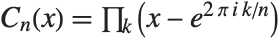 , where
  runs over all positive integers less than
  that are relatively prime to
  .
.
| Decompose[poly,x] | decompose poly, if possible, into a composition of a list of simpler polynomials |
Factorization is one important way of breaking down polynomials into simpler parts. Another, quite different, way is decomposition. When you factor a polynomial  , you write it as a product
  of polynomials
  . Decomposing a polynomial
  consists of writing it as a composition of polynomials of the form
 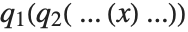 .
.
Here is a simple example of Decompose. The original polynomial  can be written as the polynomial
  , where
  is the polynomial
  :
:
Decompose recovers the original functions:
Decompose[poly,x] is set up to give a list of polynomials in x, which, if composed, reproduce the original polynomial. The original polynomial can contain variables other than x, but the sequence of polynomials that Decompose produces are all intended to be considered as functions of x.
Unlike factoring, the decomposition of polynomials is not completely unique. For example, the two sets of polynomials  and
and  , related by
  and
and  give the same result on composition, so that
  . The Wolfram Language follows the convention of absorbing any constant terms into the first polynomial in the list produced by Decompose.
| InterpolatingPolynomial[{f1,f2,…},x] | |
give a polynomial in x which is equal to fi when x is the integer i | |
| InterpolatingPolynomial[{{x1,f1},{x2,f2},…},x] | |
give a polynomial in x which is equal to fi when x is xi | |
The Wolfram Language can work with polynomials whose coefficients are in the finite field  of integers modulo a prime
  .
.
| PolynomialMod[poly,p] | reduce the coefficients in a polynomial modulo p |
| Expand[poly,Modulus->p] | expand poly modulo p |
| Factor[poly,Modulus->p] | factor poly modulo p |
| PolynomialGCD[poly1,poly2,Modulus->p] | |
find the GCD of the polyi modulo p | |
| GroebnerBasis[polys,vars,Modulus->p] | |
find the Gröbner basis modulo p | |
A symmetric polynomial in variables  is a polynomial that is invariant under arbitrary permutations of
  . Polynomials
The fundamental theorem of symmetric polynomials says that every symmetric polynomial in  can be represented as a polynomial in elementary symmetric polynomials in
  .
.
When the ordering of variables is fixed, an arbitrary polynomial  can be uniquely represented as a sum of a symmetric polynomial
  , called the symmetric part of
  , and a remainder
  that does not contain descending monomials. A monomial
 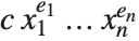 is called descending iff
  .
.
| SymmetricPolynomial[k,{x1,…,xn}] | give the |
| SymmetricReduction[f,{x1,…,xn}] | give a pair of polynomials |
| SymmetricReduction[f,{x1,…,xn},{s1,…,sn}] | |
give the pair | |
This writes the polynomial  in terms of elementary symmetric polynomials. The input polynomial is symmetric, so the remainder is zero:
Here the elementary symmetric polynomials in the symmetric part are replaced with variables  . The polynomial is not symmetric, so the remainder is not zero:
SymmetricReduction can be applied to polynomials with symbolic coefficients:
Functions like Factor usually assume that all coefficients in the polynomials they produce must involve only rational numbers. But by setting the option Extension you can extend the domain of coefficients that will be allowed.
| Factor[poly,Extension->{a1,a2,…}] | factor poly allowing coefficients that are rational combinations of the ai |
Expand gives the original polynomial back again:
| Factor[poly,Extension->Automatic] | factor poly allowing algebraic numbers in poly to appear in coefficients |
By default, Factor will not factor this polynomial:
Other polynomial functions work much like Factor. By default, they treat algebraic number coefficients just like independent symbolic variables. But with the option Extension->Automatic they perform operations on these coefficients.
By default, Cancel does not reduce these polynomials:
By default, PolynomialLCM pulls out no common factors:
| IrreduciblePolynomialQ[poly,ExtensionAutomatic] | test whether poly is an irreducible polynomial over the rationals extended by the coefficients of poly |
| IrreduciblePolynomialQ[poly,Extension->{a1,a2,…}] | test whether poly is irreducible over the rationals extended by the coefficients of poly and by a1,a2,… |
| IrreduciblePolynomialQ[poly,ExtensionAll] | test irreducibility over the field of all complex numbers |
A polynomial is irreducible over a field F if it cannot be represented as a product of two nonconstant polynomials with coefficients in F.
Over the rationals extended by Sqrt[2], the polynomial is reducible:
Over the rationals extended by Sqrt[3], the polynomial is reducible:
| TrigExpand[expr] | expand trigonometric expressions out into a sum of terms |
| TrigFactor[expr] | factor trigonometric expressions into products of terms |
| TrigFactorList[expr] | give terms and their exponents in a list |
| TrigReduce[expr] | reduce trigonometric expressions using multiple angles |
TrigExpand works on hyperbolic as well as circular functions:
TrigReduce reproduces the original form again:
The Wolfram System automatically uses functions like Tan whenever it can:
| TrigToExp[expr] | write trigonometric functions in terms of exponentials |
| ExpToTrig[expr] | write exponentials in terms of trigonometric functions |
TrigToExp writes trigonometric functions in terms of exponentials:
TrigToExp also works with hyperbolic functions:
ExpToTrig does the reverse, getting rid of explicit complex numbers whenever possible:
ExpToTrig deals with hyperbolic as well as circular functions:
You can also use ExpToTrig on purely numerical expressions:
The Wolfram Language usually pays no attention to whether variables like x stand for real or complex numbers. Sometimes, however, you may want to make transformations which are appropriate only if particular variables are assumed to be either real or complex.
The function ComplexExpand expands out algebraic and trigonometric expressions, making definite assumptions about the variables that appear.
| ComplexExpand[expr] | expand expr assuming that all variables are real |
| ComplexExpand[expr,{x1,x2,…}] | expand expr assuming that the xi are complex |
In this case, a is assumed to be real, but x is assumed to be complex, and is broken into explicit real and imaginary parts:
There are several ways to write a complex variable z in terms of real parameters. As above, for example, z can be written in the "Cartesian form" Re[z]+I Im[z]. But it can equally well be written in the "polar form" Abs[z] Exp[I Arg[z]].
The option TargetFunctions in ComplexExpand allows you to specify how complex variables should be written. TargetFunctions can be set to a list of functions from the set {Re,Im,Abs,Arg,Conjugate,Sign}. ComplexExpand will try to give results in terms of whichever of these functions you request. The default is typically to give results in terms of Re and Im.
Nested logical and piecewise functions can be expanded out much like nested arithmetic functions. You can do this using LogicalExpand and PiecewiseExpand.
| LogicalExpand[expr] | expand out logical functions in expr |
| PiecewiseExpand[expr] | expand out piecewise functions in expr |
| PiecewiseExpand[expr,assum] | expand out with the specified assumptions |
LogicalExpand puts logical expressions into a standard disjunctive normal form (DNF), consisting of an OR of ANDs.
LogicalExpand expands this into an OR of ANDs:
LogicalExpand works on all logical functions, always converting them into a standard OR of ANDs form. Sometimes the results are inevitably quite large.
Xor can be expressed as an OR of ANDs:
Any collection of nested conditionals can always in effect be flattened into a piecewise normal form consisting of a single Piecewise object. You can do this in the Wolfram Language using PiecewiseExpand.
Functions like Max and Abs, as well as Clip and UnitStep, implicitly involve conditionals, and combinations of them can again be reduced to a single Piecewise object using PiecewiseExpand.
This gives a result as a single Piecewise object:
Functions like Floor, Mod, and FractionalPart can also be expressed in terms of Piecewise objects, though in principle they can involve an infinite number of cases.
The Wolfram Language by default limits the number of cases that the Wolfram Language will explicitly generate in the expansion of any single piecewise function such as Floor at any stage in a computation. You can change this limit by resetting the value of $MaxPiecewiseCases.
| Simplify[expr] | try various algebraic and trigonometric transformations to simplify an expression |
| FullSimplify[expr] | try a much wider range of transformations |
Simplify performs the simplification:
Simplify performs standard algebraic and trigonometric simplifications:
It does not, however, do more sophisticated transformations that involve, for example, special functions:
FullSimplify does perform such transformations:
| FullSimplify[expr,ExcludedForms->pattern] | |
try to simplify expr, without touching subexpressions that match pattern | |
By default, FullSimplify will try to simplify everything:
This makes FullSimplify avoid simplifying the square roots:
| FullSimplify[expr,TimeConstraint->t] | |
try to simplify expr, working for at most t seconds on each transformation | |
| FullSimplify[expr,TransformationFunctions->{f1,f2,…}] | |
use only the functions fi in trying to transform parts of expr | |
| FullSimplify[expr,TransformationFunctions->{Automatic,f1,f2,…}] | |
use built‐in transformations as well as the fi | |
| Simplify[expr,ComplexityFunction->c] and FullSimplify[expr,ComplexityFunction->c] | |
simplify using c to determine what form is considered simplest | |
In both Simplify and FullSimplify there is always an issue of what counts as the "simplest" form of an expression. You can use the option ComplexityFunction->c to provide a function to determine this. The function will be applied to each candidate form of the expression, and the one that gives the smallest numerical value will be considered simplest.
With its default definition of simplicity, Simplify leaves this unchanged:
The Wolfram Language normally makes as few assumptions as possible about the objects you ask it to manipulate. This means that the results it gives are as general as possible. But sometimes these results are considerably more complicated than they would be if more assumptions were made.
| Refine[expr,assum] | refine expr using assumptions |
| Simplify[expr,assum] | simplify with assumptions |
| FullSimplify[expr,assum] | full simplify with assumptions |
| FunctionExpand[expr,assum] | function expand with assumptions |
Simplify by default does essentially nothing with this expression:
By applying Simplify and FullSimplify with appropriate assumptions to equations and inequalities, you can in effect establish a vast range of theorems.
Now Simplify can prove that the equation is true:
Simplify and FullSimplify always try to find the simplest forms of expressions. Sometimes, however, you may just want the Wolfram Language to follow its ordinary evaluation process, but with certain assumptions made. You can do this using Refine. The way it works is that Refine[expr,assum] performs the same transformations as the Wolfram Language would perform automatically if the variables in expr were replaced by numerical expressions satisfying the assumptions assum.
There is no simpler form that Simplify can find:
An important class of assumptions is those which assert that some object is an element of a particular domain. You can set up such assumptions using x∈dom, where the ∈ character can be entered as EscelEsc or ∖[Element].
| x∈dom or Element[x,dom] | assert that x is an element of the domain dom |
| {x1,x2,…}∈dom | assert that all the xi are elements of the domain dom |
| patt∈dom | assert that any expression that matches patt is an element of the domain dom |
| Complexes | the domain of complex numbers |
| Reals | the domain of real numbers |
| Algebraics | the domain of algebraic numbers |
| Rationals | the domain of rational numbers |
| Integers | the domain of integers |
| Primes | the domain of primes |
| Booleans |
If you say that a variable satisfies an inequality, the Wolfram Language will automatically assume that it is real:
By using Simplify, FullSimplify, and FunctionExpand with assumptions, you can access many of the Wolfram Language's vast collection of mathematical facts.
FullSimplify accesses knowledge about special functions:
The Wolfram Language knows about discrete mathematics and number theory as well as continuous mathematics.
In something like Simplify[expr,assum] or Refine[expr,assum], you explicitly give the assumptions you want to use. But sometimes you may want to specify one set of assumptions to use in a whole collection of operations. You can do this by using Assuming.
| Assuming[assum,expr] | use assumptions assum in the evaluation of expr |
| $Assumptions | the default assumptions to use |
Functions like Simplify and Refine take the option Assumptions, which specifies what default assumptions they should use. By default, the setting for this option is Assumptions:>$Assumptions. The way Assuming then works is to assign a local value to $Assumptions, much as in Block.
In addition to Simplify and Refine, a number of other functions take Assumptions options, and thus can have assumptions specified for them by Assuming. Examples are FunctionExpand, Integrate, Limit, Series, and LaplaceTransform.
The assumption is automatically used in Integrate: