

BilateralFilter
BilateralFilter[data,σ,μ]
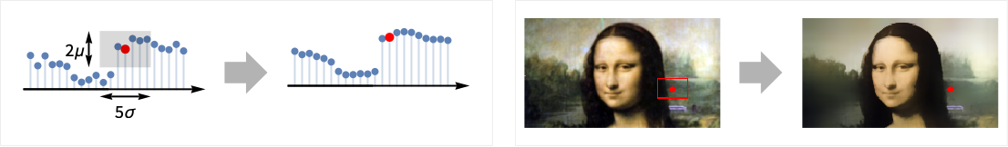
applies a bilateral filter of spatial spread σ and pixel value spread μ to data.
Details and Options
- BilateralFilter is a nonlinear local filter used for edge-preserving smoothing. The amount of smoothing is dependent on the values of σ and μ.
- BilateralFilter replaces each pixel by a weighted average of its neighbors, using normalized Gaussian matrices as weights.
- The data can be any of the following:
-
list arbitrary-rank numerical array tseries temporal data such as TimeSeries, TemporalData, … image arbitrary Image or Image3D object audio an Audio object video a Video object - When applied to multichannel audio signals and images, the Euclidean distance between channel vectors is computed.
- At the data boundaries, BilateralFilter uses smaller neighborhoods.
- The following options can be given:
-
MaxIterations 1 maximum number of iterations WorkingPrecision MachinePrecision the precision to use - BilateralFilter uses a Gaussian matrix of spatial radius 5/2 σ.
- BilateralFilter always returns an image of a real type.
- For large values of μ, bilateral filtering yields results similar to Gaussian filtering.
Background & Context
- BilateralFilter is a filter for smoothing images to remove local variations typically caused by noise, rough textures, etc. BilateralFilter is often used as a preprocessing step before doing other image analysis operations, such as segmentation. Bilateral filtering can also be used to perform unsharp masking by subtracting the filtered image from the original and then adding the original back in.
- BilateralFilter performs a nonlinear edge-preserving smoothing. The smoothing is done by replacing each pixel with a weighted average of its neighbors, where weights are taken from a normalized Gaussian distribution based on color value similarity. Here, the standard deviation σ and mean μ of the Gaussian distribution are specified as arguments.
- BilateralFilter works with arbitrary grayscale and color images, as well as with 3D and 2D images. When applied to multichannel images, BilateralFilter does not operate channel-by-channel but rather uses the Euclidean distance between channel vectors.
- Other edge-preserving filters include MeanShiftFilter and PeronaMalikFilter. Similar filters that are not edge preserving include MeanFilter and GaussianFilter. For large values of the Gaussian distribution mean, bilateral filtering yields results similar to Gaussian filtering.
Examples
open all close allBasic Examples (3)
Bilateral filtering of a vector:
BilateralFilter[ {1, 0, 1, 4, 4, 5, 2, 1}, 3, 1]Filter a TimeSeries:
ts = TemporalData[TimeSeries, {{{0., -0.054108337548928784, 0.1280211704499059, 0.28162021808461324,
    -0.2057320325139802, -0.4871901025739722, -0.7154387408784426, -0.7399660905024047,
    -0.6981022018441507, -0.7178077145466483, -0.8034462541874 ... 7894984276149, 1.8851123992920942, 1.8341759268762767, 2.0335844117979263}},
  {{0., 10., 0.1}}, 1, {"Continuous", 1}, {"Continuous", 1}, 1,
  {ValueDimensions -> 1, ResamplingMethod -> {"Interpolation", InterpolationOrder -> 1}}}, False,
10.];filtered = BilateralFilter[ts, 5, 2]ListLinePlot[{ts, filtered}, PlotLegends -> {"original data", "filtered"}]Smooth details in a color image:
BilateralFilter[[image], 7, .1]Scope (8)
Data (8)
Bilateral filtering of a list:
{ListLinePlot[data = Table[Sign[i - 1] + RandomReal[{-.2, .2}], {i, 0, 2, 0.01}]],
	ListLinePlot[BilateralFilter[data, 10, .5]]}
Bilateral filtering of a 2D array:
BilateralFilter[(| | | | |
| - | - | - | - |
| 0 | 3 | 2 | 2 |
| 3 | 9 | 9 | 6 |
| 5 | 8 | 7 | 0 |
| 3 | 1 | 1 | 2 |), 2, 2]//MatrixFormFilter a TimeSeries:
ts = TemporalData[TimeSeries, {{{0., -0.27267267057145633, -0.6672983789995302, -0.5338541947930846,
    -0.6117404489279314, -0.6755527076595494, -0.02125421294486496, -0.10792797291843935,
    -0.6138271235477938, -0.3248568606554575, -0.08843449054 ... 2053424, -0.49980440691873723, -0.5388679788215971,
    -0.4101602764645551}}, {{0, 1., 0.01}}, 1, {"Continuous", 1}, {"Continuous", 1}, 1,
  {ValueDimensions -> 1, ResamplingMethod -> {"Interpolation", InterpolationOrder -> 1}}}, False,
10.1];filtered = BilateralFilter[ts, 3, 1]ListLinePlot[{ts, filtered}, PlotLegends -> {"original data", "filtered"}]Filter an Audio signal:
a = Import["ExampleData/rule30.wav"];b = BilateralFilter[a, 25, 0.5]AudioPlot[{a, b}]Bilateral filtering smooths an image while preserving edges:
BilateralFilter[[image], 2, 0.2]BilateralFilter[Video["ExampleData/fish.mp4"], 3, .5]BilateralFilter[[image], 5, 0.1]Symbolic computation of a bilateral filter:
BilateralFilter[{a, b, c}, 1, .1]Options (6)
MaxIterations (2)
By default, one iteration of bilateral filtering is performed:
i = [image];
BilateralFilter[i, 2, .05, MaxIterations -> 1]BilateralFilter[i, 2, .05, MaxIterations -> 10]Repeatedly filter a TimeSeries:
ts = TemporalData[TimeSeries, {{{0., -0.27267267057145633, -0.6672983789995302, -0.5338541947930846,
    -0.6117404489279314, -0.6755527076595494, -0.02125421294486496, -0.10792797291843935,
    -0.6138271235477938, -0.3248568606554575, -0.08843449054 ... 2053424, -0.49980440691873723, -0.5388679788215971,
    -0.4101602764645551}}, {{0, 1., 0.01}}, 1, {"Continuous", 1}, {"Continuous", 1}, 1,
  {ValueDimensions -> 1, ResamplingMethod -> {"Interpolation", InterpolationOrder -> 1}}}, False,
10.1];filtered = BilateralFilter[ts, 3, .3, MaxIterations -> 100]ListLinePlot[{ts, filtered}, PlotLegends -> {"original data", "filtered"}]WorkingPrecision (4)
By default, MachinePrecision is used with integer arrays:
BilateralFilter[{3, 4, 4, 3, 2}, 2, 1]Perform exact computation instead:
BilateralFilter[{3, 4, 4, 3, 2}, 2, 1, WorkingPrecision -> ∞]By default, the precision of the input is used for real arrays:
BilateralFilter[{1.0000000000000000000, 2.0000000000000000000, 3.0000000000000000000, 4.0000000000000000000}, 2, 1]BilateralFilter[{1.0000000000000000000, 2.0000000000000000000, 3.0000000000000000000, 4.0000000000000000000}, 2, 1, WorkingPrecision -> MachinePrecision]With symbolic arrays, exact computation is used:
BilateralFilter[{a, b, c}, 1, 1]WorkingPrecision is ignored when filtering images:
BilateralFilter[[image], 2, .5, WorkingPrecision -> Infinity]An image of a real type is always returned:
ImageType[%]Applications (5)
BilateralFilter[[image], 2, .2]Create a posterization effect by performing multiple iterations:
BilateralFilter[[image], 2, .05, MaxIterations -> 10]Bilateral filtering with a large color spread value, used for background removal:
ImageSubtract[ #, BilateralFilter[#, 4, 0.9]] & [[image]]Bilateral filtering as a preprocessing step for image segmentation:
ClusteringComponents[BilateralFilter[[image], 4, 0.3], 5]// ColorizeUnsharp masking using bilateral filtering:
img = [image];
ImageAdd[img, ImageSubtract[img, BilateralFilter[img, 5, .2]]]
Properties & Relations (2)
Bilateral filtering performs noise reduction while preserving edges:
data = Table[Sign[i - 1] + RandomReal[{-.2, .2}], {i, 0, 2, 0.01}];
{ListLinePlot[data], ListLinePlot[BilateralFilter[data, 20, .5]]}
MeanFilter also reduces noise, but does not preserve edges:
MeanFilter[data, 20]//ListLinePlotFor large values of the Gaussian distribution mean, bilateral filtering yields results similar to Gaussian filtering:
{BilateralFilter[[image], 2, 2], GaussianFilter[[image], 5]}Text
Wolfram Research (2010), BilateralFilter, Wolfram Language function, https://reference.wolfram.com/language/ref/BilateralFilter.html (updated 2025).
CMS
Wolfram Language. 2010. "BilateralFilter." Wolfram Language & System Documentation Center. Wolfram Research. Last Modified 2025. https://reference.wolfram.com/language/ref/BilateralFilter.html.
APA
Wolfram Language. (2010). BilateralFilter. Wolfram Language & System Documentation Center. Retrieved from https://reference.wolfram.com/language/ref/BilateralFilter.html