给出矩阵 m 的 Cholesky 分解.
CholeskyDecomposition
给出矩阵 m 的 Cholesky 分解.
更多信息和选项

- 矩阵 m 可为数字矩阵或符号矩阵,但是必须为正定 Hermitian 型.
- CholeskyDecomposition[m] 生成一个满足 ConjugateTranspose[u].u==m 的上三角矩阵 u.
- 通过设置 TargetStructure->"Structured",CholeskyDecomposition[m] 可将 u 作为一个 UpperTriangularMatrix 返回.
范例
打开所有单元 关闭所有单元基本范例 (2)
CholeskyDecomposition[(| | |
| - | - |
| 2 | 1 |
| 1 | 2 |)]ConjugateTranspose[%].%//MatrixFormPositiveDefiniteMatrixQ[(| | |
| - | - |
| 2 | 1 |
| 1 | 2 |)]CholeskyDecomposition[(| | | |
| ----------------------------------------- | ----------------------------------------- | ----------------------------------------- |
| 2.4138543944035415 + 0. I | -2.4654688123131883 - 1.922250972681738 I | 1.1102409170396648 + 2.2005827949357206 I |
| -2.4654688123131883 + 1.922250972681738 I | 6.25162395665795 + 0. I | -4.11767176535921 - 1.3474244699923004 I |
| 1.1102409170396648 - 2.2005827949357206 I | -4.11767176535921 + 1.3474244699923004 I | 3.433935295685307 + 0. I |)]//MatrixFormUpperTriangularMatrixQ[%]范围 (11)
基础用法 (7)
m = {{0.5, 0.3, 0.4}, {0.3, 1.1, -0.2}, {0.4, -0.2, 0.7}};u = CholeskyDecomposition[m]m == Transpose[u].uCholeskyDecomposition[{{2, I}, {-I, 3}}]CholeskyDecomposition 将检验输入是否并非埃尔米特和正定矩阵:

m = {{2, I}, {I, 3}};
CholeskyDecomposition[m]{HermitianMatrixQ[m], PositiveDefiniteMatrixQ[m]}将 CholeskyDecomposition 用于精确矩阵:
u = CholeskyDecomposition[(| | | |
| ---- | --------- | --- |
| 5E^2 | 14 | 15 |
| 14 | Sqrt[863] | 8 |
| 15 | 8 | 18π |)]u^.u//MatrixFormRandomVariate[WishartMatrixDistribution[7, {{1, 1 / 2, 0}, {1 / 2, 2, -1 / 2}, {0, -1 / 2, 1}}], WorkingPrecision -> 15]CholeskyDecomposition[%]//MatrixForm将 CholeskyDecomposition 用于符号矩阵:
CholeskyDecomposition[(| | |
| - | - |
| a | b |
| b | a |)]FullSimplify[ConjugateTranspose[%].%, a > b && a > -b]Eigenvalues[(| | |
| - | - |
| a | b |
| b | a |)]A = RandomReal[1, {1000, 1000}];
mat = A.A^;AbsoluteTiming[CholeskyDecomposition[mat];]实对称正定 CenteredInterval 矩阵的 Cholesky 分解:
rm = Map[CenteredInterval, RandomReal[{-10, 10}, {3, 3}, WorkingPrecision -> 10], {2}];
(m = rm.Transpose[rm])//MatrixForm(q = CholeskyDecomposition[m])//MatrixFormMapThread[IntervalMemberQ, {Transpose[q].q, m}, 2]//MatrixForm特殊矩阵 (4)
CholeskyDecomposition[SparseArray[Automatic, {5, 5}, 0,
{1, {{0, 5, 10, 15, 20, 25}, {{1}, {2}, {3}, {4}, {5}, {1}, {2}, {3}, {4}, {5}, {1}, {2}, {3},
{4}, {5}, {1}, {2}, {3}, {4}, {5}, {2}, {3}, {4}, {5}, {1}}},
{3, 3, 3, 2, 1, 3, 4, 4, 3, 2, 3, 4, 5, 4, 3, 2, 3, 4, 4, 3, 2, 3, 3, 3, 1}}]]//MatrixForm%.% == SparseArray[Automatic, {5, 5}, 0,
{1, {{0, 5, 10, 15, 20, 25}, {{1}, {2}, {3}, {4}, {5}, {1}, {2}, {3}, {4}, {5}, {1}, {2}, {3},
{4}, {5}, {1}, {2}, {3}, {4}, {5}, {2}, {3}, {4}, {5}, {1}}},
{3, 3, 3, 2, 1, 3, 4, 4, 3, 2, 3, 4, 5, 4, 3, 2, 3, 4, 4, 3, 2, 3, 3, 3, 1}}]SymmetrizedArray[{{1, 1} -> 5, {2, 2} -> 3, {3, 1} -> 2, {3, 3} -> 1}, {3, 3}, Symmetric[All]]CholeskyDecomposition[%]用于 QuantityArray 结构化矩阵:
QuantityArray[{{1, 2}, {2, 5}}, "Meters"]CholeskyDecomposition[%]CholeskyDecomposition[IdentityMatrix[3]]HilbertMatrix 的乔里斯基分解:
m = HilbertMatrix[5];CholeskyDecomposition[m]//MatrixForm选项 (1)
TargetStructure (1)
设置 TargetStructure->"Dense",结果会以稠密矩阵的形式给出:
CholeskyDecomposition[(| | | | |
| - | - | - | - |
| 1 | 1 | 1 | 1 |
| 1 | 2 | 2 | 2 |
| 1 | 2 | 3 | 3 |
| 1 | 2 | 3 | 4 |), TargetStructure -> "Dense"]设置 TargetStructure->"Structured",结果会以 UpperTriangularMatrix 的形式给出:
CholeskyDecomposition[(| | | | |
| - | - | - | - |
| 1 | 1 | 1 | 1 |
| 1 | 2 | 2 | 2 |
| 1 | 2 | 3 | 3 |
| 1 | 2 | 3 | 4 |), TargetStructure -> "Structured"]应用 (2)
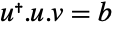
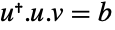
三角线性方程组是一个线性方程组,其中第一个方程有一个变量,而随后的每个方程正好引入一个附加变量. 将以下三变量方程组改写为两个六变量三角线性方程组:
system = {3 x - y + z == 3, -x + 3 y == 5, x + 3 z == 7};v = {x, y, z};
m = {{3, -1, 1}, {-1, 3, 0}, {1, 0, 3}};
b = {3, 5, 7};
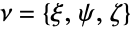
u = CholeskyDecomposition[m]system == Thread[u.u.v == b]ν = {ξ, ψ, ζ};
tri1 = Reverse[Thread[u.v == ν]];
Column[tri1]tri2 = Thread[u.ν == b];
Column[tri2]v /. Solve[Join[tri1, tri2], Join[v, ν]]SolveValues[system, v]乔里斯基分解可用于从许多独立随机值创建具有指定协方差的随机样本,例如蒙特卡罗模拟. 从所需的协方差矩阵开始,计算下三角矩阵
,其中
是乔里斯基分解:
cov = (| | | |
| ------------------- | ------------------- | ------------------- |
| 0.5679913970339641 | 0.13175676534111222 | 0.22467465390992986 |
| 0.13175676534111222 | 0.7257156525584264 | 0.685100031070936 |
| 0.22467465390992986 | 0.685100031070936 | 2.64673926689887 |);
l = CholeskyDecomposition[cov]rand = l.#& /@ RandomVariate[NormalDistribution[], {10 ^ 6, 3}];Covariance[rand]//MatrixForm//NumberForm[#, 3]&属性和关系 (7)
m = {{4, 3, 2, 1}, {3, 4, 3, 2}, {2, 3, 4, 3}, {1, 2, 3, 4}};
HermitianMatrixQ[m] && PositiveDefiniteMatrixQ[m]u = CholeskyDecomposition[m]验证 ConjugateTranspose[u].u == m:
ConjugateTranspose[u].u == mCholeskyDecomposition[m] 是上三角和正定矩阵:
CholeskyDecomposition[{{3, 2, 1}, {2, 3, 2}, {1, 2, 3}}]UpperTriangularMatrixQ[%] && PositiveDefiniteMatrixQ[%]c = CholeskyDecomposition[{{3, 2, 1}, {2, 3, 2}, {1, 2, 3}}]s = MatrixFunction[Sqrt, {{3, 2, 1}, {2, 3, 2}, {1, 2, 3}}]//FullSimplifyHermitianMatrixQ[s]{FullSimplify[Det[c] == Det[s]], PositiveDefiniteMatrixQ[s], PositiveDefiniteMatrixQ[c]}对于实数矩阵
,
的乔里斯基分解与
的 QR 分解直到符号都一致:
m = RandomReal[1, {6, 3}];求 Transpose[m].m 的乔里斯基分解:
u = CholeskyDecomposition[Transpose[m].m];计算 QRDecomposition[m]:
{q, r} = QRDecomposition[m];Chop[r Sign[Tr[r, List]] - u]m = RandomComplex[1 + I, {6, 3}];求 ConjugateTranspose[m].m 的 Cholesky 分解:
u = CholeskyDecomposition[ConjugateTranspose[m].m];计算 QRDecomposition[m]:
{q, r} = QRDecomposition[m];Chop[r Sign[Tr[r, List]] - u]对于埃尔米特矩阵,LDLDecomposition 给出一对
,使得 l 是下三角矩阵,d 是对角矩阵,并且原矩阵等于
:
m0 = RandomComplex[1 + I, {6, 3}];
m = ConjugateTranspose[m0].m0;
{l, d} = LDLDecomposition[m]对于正定矩阵,可以通过
.
从 LDLDecomposition 恢复 Cholesky 分解:
c1 = Sqrt[d].ConjugateTranspose[l];
c1 == CholeskyDecomposition[m]CholeskyDecomposition 是一种 LU 分解:
h = {{2, 1}, {1, 2}};
MatrixForm[u = CholeskyDecomposition[h]]MatrixForm[l = ConjugateTranspose[u]]l.u == h这通常是一个与 LUDecomposition 给出的分解不同的分解:
MatrixForm /@ Take[LUDecomposition[h], 2]可能存在的问题 (2)
Head[CholeskyDecomposition[N[HilbertMatrix[16]]]]
N[Eigenvalues[HilbertMatrix[16]]]Head[CholeskyDecomposition[N[HilbertMatrix[16], 24]]]s = Block[{n = 500}, SparseArray[{{i_, i_} -> 2.n ^ 2 - 1., {i_, j_} /; Abs[i - j] == 1 -> -1.n ^ 2}, {n, n}]]即便结果为稀疏的,还是将 Cholesky 分解作为稠密矩阵计算:
u = CholeskyDecomposition[s];
ArrayPlot[u]用 LinearSolve 将得到一个有着稀疏 Cholesky 因式分解的 LinearSolveFunction:
f = LinearSolve[s, Method -> "Cholesky"]N[ByteCount[u] / ByteCount[f]]技术笔记
-
▪
- 高级矩阵运算
历史
2003年引入 (5.0) | 在以下年份被更新:2023 (13.3) ▪ 2024 (14.0)
文本
Wolfram Research (2003),CholeskyDecomposition,Wolfram 语言函数,https://reference.wolfram.com/language/ref/CholeskyDecomposition.html (更新于 2024 年).
CMS
Wolfram 语言. 2003. "CholeskyDecomposition." Wolfram 语言与系统参考资料中心. Wolfram Research. 最新版本 2024. https://reference.wolfram.com/language/ref/CholeskyDecomposition.html.
APA
Wolfram 语言. (2003). CholeskyDecomposition. Wolfram 语言与系统参考资料中心. 追溯自 https://reference.wolfram.com/language/ref/CholeskyDecomposition.html 年
BibTeX
@misc{reference.wolfram_2026_choleskydecomposition, author="Wolfram Research", title="{CholeskyDecomposition}", year="2024", howpublished="\url{https://reference.wolfram.com/language/ref/CholeskyDecomposition.html}", note=[Accessed: 04-September-2026]}
BibLaTeX
@online{reference.wolfram_2026_choleskydecomposition, organization={Wolfram Research}, title={CholeskyDecomposition}, year={2024}, url={https://reference.wolfram.com/language/ref/CholeskyDecomposition.html}, note=[Accessed: 04-September-2026]}