Wolfram 语言与系统参考资料中心

FindMinimum

FindMinimum[f,x]

搜索 f 的局部极小值，从一个自动选定的点开始.

FindMinimum[f,{x,x₀}]

搜索 f 的局部最小值，从 x=x₀ 开始.

FindMinimum[f,{{x,x₀},{y,y₀},…}]

搜索多元函数的局部最小值.

FindMinimum[{f,cons},{{x,x₀},{y,y₀},…}]

搜索约束条件 cons 下局部最小值.

FindMinimum[{f,cons},{x,y,…}]

从约束条件定义区域内的点开始.

FindMinimum

FindMinimum[f,x]

搜索 f 的局部极小值，从一个自动选定的点开始.

FindMinimum[f,{x,x₀}]

搜索 f 的局部最小值，从 x=x₀ 开始.

FindMinimum[f,{{x,x₀},{y,y₀},…}]

搜索多元函数的局部最小值.

FindMinimum[{f,cons},{{x,x₀},{y,y₀},…}]

搜索约束条件 cons 下局部最小值.

FindMinimum[{f,cons},{x,y,…}]

从约束条件定义区域内的点开始.

范例

打开所有单元关闭所有单元

基本范例 (4)

搜索一个局部最小值，从开始搜索：

Wolfram Language code: FindMinimum[x Cos[x], {x, 2}]

Wolfram Language code: Plot[x Cos[x], {x, 0, 20}]

提取在局部最小值处 x 的值：

Wolfram Language code: x /. Last[FindMinimum[x Cos[x], {x, 2}]]

求局部最小值，从开始，在约束条件下：

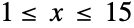
Wolfram Language code: FindMinimum[{x Cos[x], 1 ≤ x ≤ 15}, {x, 7}]

求一个线性函数的最小值，在线性和整数约束下：

Wolfram Language code: FindMinimum[{x + y, x + 2y ≥ 3 && x ≥ 0 && y ≥ 0 && y∈Integers}, {x, y}]

在几何区域上求函数的最小值：

Wolfram Language code: FindMinimum[{x + y, {x, y}∈Disk[]}, {x, y}]

绘制图线：

Wolfram Language code: Show[ContourPlot[x + y, {x, y}∈Disk[]], Graphics[{Red, PointSize[Large], Point[{x, y} /. Last[%]]}]]

范围 (12)

不同的初始值，您可以获得不同的局部最小值:

Wolfram Language code: FindMinimum[x Cos[x], {x, 5}]

Wolfram Language code: FindMinimum[x Cos[x], {x, 10}]

一个二元函数的局部最小值，从 x=2，y=2 开始：

Wolfram Language code: FindMinimum[Sin[x]Sin[2y], {{x, 2}, {y, 2}}]

限制在一个圆盘内的局部最小值：

Wolfram Language code: FindMinimum[{Sin[x]Sin[2y], x ^ 2 + y ^ 2 < 3}, {{x, 2}, {y, 2}}]

不一定要提供初始值：

Wolfram Language code: FindMinimum[{Sin[x ]Sin[2y], x ^ 2 + y ^ 2 < 3}, {x, y}]

对线性目标和约束条件，可以加上整数约束条件：

Wolfram Language code: FindMinimum[{x + y, 3x + 2y ≥ 7 && x ≥ 0 && y ≥ 0}, {x, y}]

Wolfram Language code: FindMinimum[{x + y, 3x + 2y ≥ 7 && x ≥ 0 && y ≥ 0 && x∈Integers}, {x, y}]

可以指定 Or 约束条件：

Wolfram Language code: FindMinimum[{x + y, x ^ 2 + y ^ 2 ≤ 1 || (x + 2) ^ 2 + (y + 2) ^ 2 ≤ 1}, {x, y}]

在区域上求最小值：

Wolfram Language code:

t = RotationTransform[{{0, 0, 1}, {1, 1, 1}}];
ℛ = TransformedRegion[Ellipsoid[{0, 0, 0}, {1, 2, 3}], t];

Wolfram Language code: FindMinimum[{z, {x, y, z}∈ℛ}, {x, y, z}]

绘制图线：

Wolfram Language code:

Graphics3D[{{Opacity[0.5], Green, GeometricTransformation[Ellipsoid[{0, 0, 0}, {1, 2, 3}], t]}, {Red, PointSize[Large], Point[{x, y, z} /. Last[%]]}}]

求两个区域之间的最小距离：

Wolfram Language code:

Subscript[ℛ, 1] = Disk[];
Subscript[ℛ, 2] = InfiniteLine[{{-2, 0}, {0, 2}}];

Wolfram Language code: FindMinimum[{(x - u)^2 + (y - v)^2, {{x, y}∈Subscript[ℛ, 1], {u, v}∈Subscript[ℛ, 2]}}, {x, y, u, v}]

绘制图线：

Wolfram Language code: Graphics[{{LightBlue, Subscript[ℛ, 1]}, {Green, Subscript[ℛ, 2]}, {Red, Point[{{x, y}, {u, v}} /. Last[%]]}}]

求最小的使得三角形和椭圆形仍然交叠：

Wolfram Language code:

Subscript[ℛ, 1] = Triangle[{{0, 0}, {1, 0}, {0, 1}}];
Subscript[ℛ, 2] = Disk[{1, 1}, {2r, r}];

Wolfram Language code: FindMinimum[{r, {x, y}∈Subscript[ℛ, 1] && {x, y}∈Subscript[ℛ, 2]}, {r, x, y}]

绘制图线：

Wolfram Language code: Graphics[{{LightBlue, Subscript[ℛ, 1], Subscript[ℛ, 2]}, {Red, Point[{x, y}]}} /. Last[%]]

求包括给定三个点的具有最小半径的圆盘：

Wolfram Language code: Subscript[ℛ, 3] = Disk[{a, b}, r];

Wolfram Language code: FindMinimum[{r, ({0, 0} | {1, 0} | {0, 1})∈Subscript[ℛ, 3]}, {a, b, r}]

绘制图线：

Wolfram Language code: Graphics[{{LightBlue, Subscript[ℛ, 3]} /. %[[2]], {Red, Point[{{0, 0}, {1, 0}, {0, 1}}]}}]

使用 Circumsphere 直接给出相同结果：

Wolfram Language code: Circumsphere[{{0, 0}, {1, 0}, {0, 1}}]//N

使用指定是中的一个向量：

Wolfram Language code: ℛ = Sphere[];

Wolfram Language code: FindMinimum[{x.{1, 2, 3}, x∈ℛ}, x]

求两个区域之间的最小距离：

Wolfram Language code:

Subscript[ℛ, 1] = Triangle[{{0, 0}, {1, 0}, {0, 1}}];
Subscript[ℛ, 2] = Disk[{2, 2}, 1];

Wolfram Language code: FindMinimum[{EuclideanDistance[x, y], {x∈Subscript[ℛ, 1], y∈Subscript[ℛ, 2]}}, {x, y}]

绘制图线：

Wolfram Language code: Graphics[{{LightBlue, Subscript[ℛ, 1], Subscript[ℛ, 2]}, {Red, Point[{x, y}]}} /. %[[2]]]

选项 (7)

AccuracyGoal 和 PrecisionGoal (2)

这指定了收敛规则和：

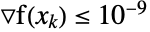
Wolfram Language code: FindMinimum[Sin[x / 2], {x, 1}, AccuracyGoal -> 9, PrecisionGoal -> 8]

这强加了收敛规则和：

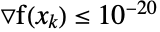
Wolfram Language code: FindMinimum[Sin[x / 2], {x, 1}, AccuracyGoal -> 20, PrecisionGoal -> 18]

设置一个高 WorkingPrecision 使过程收敛：

Wolfram Language code: FindMinimum[Sin[x / 2], {x, 1}, AccuracyGoal -> 20, PrecisionGoal -> 18, WorkingPrecision -> 40]

EvaluationMonitor (1)

绘制收敛于局部最小值：

Wolfram Language code: ListPlot[Last[Reap[FindMinimum[x Cos[x], {x, 2}, EvaluationMonitor :> Sow[x]]]]]

Gradient (1)

使用一个给定的梯度；自动地计算海森矩阵：

Wolfram Language code: FindMinimum[Sin[x]Sin[2 y], {x, y}, Gradient -> {Cos[x] Sin[2 y], 2 Cos[2 y] Sin[x]}, Method -> "Newton"]

同时提供梯度和海森矩阵：

Wolfram Language code:

FindMinimum[Sin[x]Sin[2y], {x, y}, Gradient -> {Cos[x] Sin[2 y], 2 Cos[2 y] Sin[x]}, Method -> {"Newton", Hessian -> {{-Sin[x] Sin[2 y], 2 Cos[x] Cos[2 y]}, {2 Cos[x] Cos[2 y], -4 Sin[x] Sin[2 y]}}}]

Method (1)

在这个例子中，用默认的基于导数的方式会有困难:

Wolfram Language code: FindMinimum[Abs[x + 1] + Abs[x + 1.01] + Abs[y + 1], {x, y}]

Wolfram Language code: FindMinimum[Abs[x + 1] + Abs[x + 1.01] + Abs[y + 1], {x, y}, Method -> "ConjugateGradient"]

在这些例子中，不需要导数的直接搜索方式会很有帮助:

Wolfram Language code: FindMinimum[Abs[x + 1] + Abs[x + 1.01] + Abs[y + 1], {x, y}, Method -> "PrincipalAxis"]

NMinimize 也使用了一系列的直接搜索方法：

Wolfram Language code: NMinimize[{Abs[x + 1] + Abs[x + 1.01] + Abs[y + 1], 0 > x > -2}, {x, y}]

StepMonitor (1)

在求一个函数最小值的过程中 FindMinimum 采用的步骤：

Wolfram Language code:

pts = Reap[FindMinimum[(1 - x) ^ 2 + 100(-x ^ 2 - y) ^ 2 + 1, {{x, -1.2}, {y, 1}}, StepMonitor :> Sow[{x, y}]]][[2, 1]];
pts  = Join[{{-1.2, 1}}, pts];

Wolfram Language code:

ContourPlot[(1 - x) ^ 2 + 100(-x ^ 2 - y) ^ 2 + 1//Log, {x, -1.3, 1.5}, {y, -1.5, 1.4}, Epilog -> {Red, Line[pts], Point[pts]}]

WorkingPrecision (1)

设置工作精度为；默认情况下 AccuracyGoal 和 PrecisionGoal 设置为：

Wolfram Language code: FindMinimum[Cos[x ^ 2 - 3 y] + Sin[x ^ 2 + y ^ 2], {x, y}, Method -> "Newton", WorkingPrecision -> 20]

应用 (3)

从1973年到1994年，S&P 500 指数的长期债券的年回报（R）：

Wolfram Language code:

R = {{0.942, 1.02, 1.056, 1.175, 1.002, 0.982, 0.978, 0.947, 1.003, 1.465, 0.985, 1.159, 1.366, 1.309, 0.925, 1.086, 1.212, 1.054, 1.193, 1.079, 1.217, 0.889}, {0.852, 0.735, 1.371, 1.236, 0.926, 1.064, 1.184, 1.323, 0.949, 1.215, 1.224, 1.061, 1.316, 1.186, 1.052, 1.165, 1.316, 0.968, 1.304, 1.076, 1.1, 1.012}};

计算回报的均值和协方差：

Wolfram Language code: μ = Mean[Transpose@R]

Wolfram Language code: Σ = Covariance[Transpose[R]]

Wolfram Language code: X = Map[Subscript[x, #]&, {"long T-bond", "SP500"}]

最小化波动，实现至少 10% 的回报：

Wolfram Language code: FindMinimum[{X.Σ.X, Total[X] == 1 && μ.X ≥ 1.10 && Apply[And, Thread[X ≥ {0, 0}]]}, X]

找出能包含个给定半径的不重叠圆的最小正方形，其中 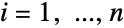. 指定圆的数量和每个圆的半径：

Wolfram Language code:

n = 20;
r = BlockRandom[RandomReal[{0.5, 1.5}, n], RandomSeeding -> 123];

若为圆的中心，则目标是最小化 . 目标可以转换为最小化和：

Wolfram Language code: objectiveConstraint = Table[-s <= Norm[c[i], Infinity] + r[[i]] <= s, {i, n}];

这些圆不能重叠：

Wolfram Language code:

nonOverlapConstraint = Table[Norm[c[i] - c[j]] >= r[[i]] + r[[j]], 
	{i, 1, n}, {j, i + 1, n}];

收集变量：

Wolfram Language code: vars = Append[Table[Element[c[i], Vectors[2, Reals]], {i, n}], Element[s, Reals]];

最小化目标：

Wolfram Language code: Short[res = FindMinimum[{s, objectiveConstraint, nonOverlapConstraint}, vars], 5]

这些圆包含在正方形中：

Wolfram Language code:

Graphics[{Table[Circle[c[i], r[[i]]], {i, n}], {FaceForm[None], EdgeForm[Black], Rectangle[{-s, -s}, {s, s}]}}] /. res[[2]]

计算圆所覆盖的面积占正方形面积的比例：

Wolfram Language code: Sum[Area[Disk[c[i], r[[i]]]], {i, n}] / Area[Rectangle[{-s, -s}, {s, s}]] /. res[[2]]

求一条穿过圆形障碍物的路径，使起点和终点之间的距离最小：

Wolfram Language code:

p = {{2, 2}, {7, 6}, {3, 5}, {4, 8}, {8, 9}, {6, 2.5}};
r = {1, 1.3, 1.5, 1, 0.7, 1.5};
{start, end} = {{0, 0}, {10, 10}};
domain = Graphics[{MapThread[Circle[#1, #2]&, {p, r}], 
	{PointSize[0.02], Point[{start, end}]}}, Frame -> True]

路径被离散成个不同的点，点与点之间的距离为，其中是最小化的轨迹长度：

Wolfram Language code:

n = 30;
distanceConstraints = Table[Inactive[Norm][x[i] - x[i - 1]] <= l / n, {i, n}];

这些点不能在圆形物体内：

Wolfram Language code: objectConstraints = Table[Inactive[Norm][-p[[j]] + x[i]] >= r[[j]], {i, 1, n}, {j, 1, 6}];

起点和终点是已知的：

Wolfram Language code: positionConstraints = {x[0] == start, x[n] == end};

收集变量：

Wolfram Language code: vars = Append[Table[x[i]∈Vectors[2, Reals], {i, 0, n}], l∈Reals];

在约束条件下，使长度最小化：

Wolfram Language code:

Short[res = FindMinimum[{l, distanceConstraints, 
	objectConstraints, positionConstraints}, vars], 2]

可视化结果：

Wolfram Language code:

pts = vars[[1 ;; -2, 1]] /. res[[2]];
Show[domain, Graphics[{Red, Point[pts]}]]

属性和关系 (2)

FindMinimum 尽可能返回一个局部最小值，NMinimize 试图求一个全局最小值：

Wolfram Language code:

objective = -100 / ((x - 1)^2 + (y - 1)^2 + 1) - 200 / ((x + 1)^2 + (y + 2)^2 + 1);
FindMinimum[{objective, x^2 + y^2 > 3 }, {{x, 2}, y}]

Wolfram Language code: NMinimize[{objective, x^2 + y^2 > 3 }, {x, y}]

Wolfram Language code: ContourPlot[objective, {x, -3, 2}, {y, -3, 2}, ...]

Minimize 求全局最小值，并可以在无穷精度下计算：

Wolfram Language code: Minimize[{-100 / ((x - 1)^2 + (y - 1)^2 + 1) - 200 / ((x + 1)^2 + (y + 2)^2 + 1), x^2 + y^2 > 3 }, {x, y}]

Wolfram Language code: N[%]

FindMinimum 同时给出最小值和产生最小值的点：

Wolfram Language code: FindMinimum[{x - 2y, x ^ 2 + y ^ 2 ≤ 1}, {x, y}]

FindArgMin 给出最小值的位置：

Wolfram Language code: FindArgMin[{x - 2y, x ^ 2 + y ^ 2 ≤ 1}, {x, y}]

FindMinValue 给出最小值：

Wolfram Language code: FindMinValue[{x - 2y, x ^ 2 + y ^ 2 ≤ 1}, {x, y}]

可能存在的问题 (6)

用机器精度算术，即使具有平滑最小值的函数看起来也会崎岖不平的：

Wolfram Language code: opt = FindMinimum[x Cos[x], {x, 1}]

Wolfram Language code:

yopt = First[opt];
xopt = x /. Last[opt];

Wolfram Language code: Plot[x Cos[x] - yopt, Evaluate[{x, xopt - 1.*^-7, xopt + 1.*^-7}], PlotRange -> All]

超出机器精度通常可以避免这类的问题：

Wolfram Language code: FindMinimum[x Cos[x], {x, 1}, WorkingPrecision -> 30]

如果限定区域为空，算法不会收敛：

Wolfram Language code: FindMinimum[{x + y, x ^ 2 + y ^ 2 ≥ 2 && x ^ 2 + y ^ 2 ≤ 1}, {x, y}]

如果最小值不是有限的，算法不会收敛：

Wolfram Language code: FindMinimum[Tan[x], {x, 2}]

Wolfram Language code: FindMinimum[{-x ^ 2 - y ^ 2, x ^ 2 + y ^ 2 > 10}, {x, y}]

整数线性规划算法仅对机器数问题有效：

Wolfram Language code: FindMinimum[{x + y, x + 2y ≥ 3 && x > 1 && y > 1 && x∈Integers}, {x, y}, WorkingPrecision -> 20]

某些时候提供一个适当的初始值可以帮助算法收敛：

Wolfram Language code: FindMinimum[{Cos[x] - Exp[(x - 0.5) y], x ^ 2 + y ^ 2 < 1}, {x, y}]

Wolfram Language code: FindMinimum[{Cos[x] - Exp[(x - 0.5) y], x ^ 2 + y ^ 2 < 1}, {{x, -1}, {y, -1}}]

符号计算函数可能很耗时：

Wolfram Language code: f[x_] := Nest[Sin[# + Sin[2#]]&, x, 15]

Wolfram Language code: FindMinimum[f[x], {x, 0}]//Timing

限制函数定义可防止符号计算：

Wolfram Language code: g[x_ ? NumericQ] := Nest[Sin[# + Sin[2#]]&, x, 15]

Wolfram Language code: FindMinimum[g[x], {x, 0}]//Timing

Top

	lhs==rhs	方程
	lhs>rhs 或 lhs>=rhs	不等式
	{x,y,…}∈reg	区域规范

AccuracyGoal	Automatic	搜索的准确度
EvaluationMonitor	None	当 f 计算时，计算的表达式
Gradient	Automatic	f 梯度分量的列表
MaxIterations	Automatic	使用最大迭代数
Method	Automatic	使用的方法
PrecisionGoal	Automatic	搜索的精度
StepMonitor	None	每个步骤计算的表达式
WorkingPrecision	MachinePrecision	内部计算的精度

更多学习资源

技术支持

数据科学、金融与商业

工程

科学与技术

教育科技

教育举措

开始

提高你的技能

与我们合作

成人教育计划

青少年教育计划

欢迎阅读

FindMinimum

更多信息和选项

范例

基本范例 (4)

范围 (12)

选项 (7)

AccuracyGoal 和 PrecisionGoal (2)

EvaluationMonitor (1)

Gradient (1)

Method (1)

StepMonitor (1)

WorkingPrecision (1)

应用 (3)

属性和关系 (2)

可能存在的问题 (6)

文本

CMS

APA

BibTeX

BibLaTeX

FindMinimum

更多信息和选项

范例

基本范例 (4)

范围 (12)

选项 (7)

AccuracyGoal 和 PrecisionGoal (2)

EvaluationMonitor (1)

Gradient (1)

Method (1)

StepMonitor (1)

WorkingPrecision (1)

应用 (3)

属性和关系 (2)

可能存在的问题 (6)

参见

技术笔记

相关指南

相关链接

历史

文本

CMS

APA

BibTeX

BibLaTeX