

Hue
詳細
- Hueは,HSB(色相,彩度,明度)あるいはHSV(色相,彩度値)としても知られている.
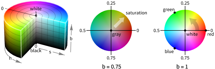
- Hueは,一般に色パラメータの簡単な解釈を許容する色の選択に使われる,RGBColorの円柱変換に対応する.
- パラメータ h,s,b そして a は,すべて0から1の範囲になくてはならない.範囲外の s,b それに a の値は切り捨てられる.この範囲外にある h の値は循環的に取り扱われる. »
- h が0から1へと変化するにつれて対応するHue[h]の色は赤,黄,シアン,青,マゼンタと変化して,ふたたび赤に戻る. »
- Hue[color]を使って任意のColorQ式をHSBに変換することができる.
- Hue["htmlcolor"]を使ってHSB空間におけるHTML色"htmlcolor"を表すことができる.
- 不透明度が指定されていなければ,Hue[h,s,b]はHue[h,s,b,1]に等しい.
- Hue[h,s,b,a]は{Hue[h,s,b],Opacity[a]}に等しい.
- Hue[h]はHue[h,1,1]と同じである. »
- 代替形のHue[{h,s,b}]およびHue[{h,s,b,a}]も使うことができる. »
- 白黒の出力デバイスでは,明度の値に基づいたグレーレベルが使われる.
- ColorConvertを使ってHueを他の色空間に変換することができる.
- 色には次のラッパーを使うことができる.
-
ColorsNear[color,…] color の周りの領域を指定する Directive[…,color,…] 色を他の指示子との組合せで指定する Glow[color] 照明とは雨関係に色を指定する » Opacity[a,color] 不透明度が a の色を指定する Style[expr,color] expr を指定の色で表示する » - 3Dの表面では,明示的なHue指示子で表面の色を指定する.最終的な陰影付けは照明に依存する.
例題
すべて開く すべて閉じる例 (4)
Graphics[{Hue[1], Disk[]}]Graphics3D[{Hue[1 / 3, 1, 1, .5], Sphere[]}]Style[x ^ 2 + y ^ 2, Hue[5 / 6]]Plot[Sin[x ^ 2], {x, 0, 2Pi}, PlotStyle -> Hue[5 / 6, 1, 1 / 2]]スコープ (3)
三次元の色 (1)
色の操作 (2)
Blendを使って2つ以上の色を混ぜる:
{Graphics[{Hue[0], Disk[]}],
	Graphics[{Blend[{Hue[0], Hue[2 / 3]}], Disk[]}],
Graphics[{Hue[2 / 3], Disk[]}]}LighterとDarkerを使ってそれぞれに白と黒を混ぜる:
{Graphics[{Lighter[Hue[1], .4], Disk[]}],
	Graphics[{Hue[1], Disk[]}],
	Graphics[{Darker[Hue[1], .4], Disk[]}]}
一般化と拡張 (3)
{Graphics[{Hue[1 / 8], Disk[]}], Graphics[{Hue[1 / 8, 1, 1], Disk[]}]}Map[Graphics[{Hue[#], Disk[]}]&, {{1, 1, 1}, {1 / 2, 1, 1}, {1 / 4, 1, 1}}]Table[Graphics[{Hue[0.08], Disk[{1, 0}], Opacity[a], Hue[1], Disk[]}], {a, 0, 1, .33}]不透明度の引数をHueに直接使う:
Table[Graphics[{Hue[.08], Disk[{1, 0}], Hue[1, 1, 1, a], Disk[]}], {a, 0, 1, .33}]アプリケーション (8)
可視化 (3)

Table[Graphics[Table[{Hue[k / n], Disk[{Cos[k 2Pi / n], Sin[k 2Pi / n]}, 1 / 2]}, {k, 0, n - 1}], PlotRange -> {{-2, 2}, {-2, 2}}], {n, 2, 8, 2}]Plot[Abs[Exp[2I x - x ^ 2 / 2]], {x, -4, 4}, Filling -> Axis, FillingStyle -> Automatic, ColorFunction -> Function[{x, y}, Hue[Rescale[Arg[Exp[2I x - x ^ 2 / 2]], {-Pi, Pi}]]], ColorFunctionScaling -> False]Plot3D[Abs[Sin[x + I y]], {x, -2Pi, 2Pi}, {y, -Pi / 2, Pi / 2}, ColorFunction -> Function[{x, y, z}, Hue[Rescale[Arg[Sin[x + I y]], {-Pi, Pi}]]], ColorFunctionScaling -> False, PlotStyle -> Opacity[0.8], Mesh -> False]HSBカラーモデル (5)
RGB立方体からISO色相曲面をプロットする. 色相は,0 (赤),1/6(黄),2/6(緑),3/6(シアン),4/6(青),5/6(マゼンタ)である.原色は,0の赤,1/3の緑,2/3の青である.二次色は,2つの原色を混ぜたもので,例えば1/6の黄色は赤と緑を等分に混ぜたものである:
Table[ParametricPlot3D[List@@ColorConvert[Hue[h, s, b], RGBColor], {s, 0, 1}, {b, 0, 1}, ColorFunction -> Function[{x, y, z}, RGBColor[x, y, z]], Lighting -> "Neutral", Mesh -> None, Axes -> False, PlotLabel -> h, ImageSize -> Tiny], {h, {0, 1 / 6, 2 / 6, 3 / 6, 4 / 6, 5 / 6}}]色相成分をインタラクティブに操作すると,上記の理解が簡単になる:
Manipulate[ParametricPlot3D[List@@ColorConvert[Hue[h, s, b], RGBColor], {s, 0, 1}, {b, 0, 1}, ColorFunction -> Function[{x, y, z}, RGBColor[x, y, z]], Lighting -> "Neutral", Mesh -> None, Axes -> False, PlotLabel -> h], {h, 0, 1}]RGB立方体からISO彩度曲面をプロットする.結果として得られるISO彩度曲面は六角錘で,HSBモデルは六角錘モデルとしても知られている:
Table[ParametricPlot3D[List@@ColorConvert[Hue[h, s, b], RGBColor], {h, 0, 1}, {b, 0, 1}, ColorFunction -> Function[{x, y, z}, RGBColor[x, y, z]], Lighting -> "Neutral", Mesh -> None, Axes -> False, PlotLabel -> s, ImageSize -> Tiny, PlotRange -> {0, 1}], {s, {0.1, 0.3, 0.5, 1.0}}]RGBColor[r,g,b]の彩度は(Max[r,g,b]-Min[r,g,b])/Max[r,g,b]で得られる.彩度0は灰色の線,つまり 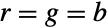 に相当する:
Reduce[(Max[r, g, b] - Min[r, g, b]) / Max[r, g, b] == 0 && 0 ≤ r ≤ 1 && 0 ≤ g ≤ 1 && 0 ≤ b ≤ 1, {r, g, b}]彩度1は(上記から分かるように) ,
 ,
 のいずれかの曲面である:
Reduce[(Max[r, g, b] - Min[r, g, b]) / Max[r, g, b] == 1 && 0 ≤ r ≤ 1 && 0 ≤ g ≤ 1 && 0 ≤ b ≤ 1, {r, g, b}, Backsubstitution -> True]Manipulate[ParametricPlot3D[List@@ColorConvert[Hue[h, s, b], RGBColor], {h, 0, 1}, {b, 0, 1}, ColorFunction -> Function[{x, y, z}, RGBColor[x, y, z]], Lighting -> "Neutral", Mesh -> None, Axes -> False, PlotLabel -> s, PlotRange -> {0, 1}], {{s, 0.3}, 0, 1}]ISO明度曲面をプロットする.RGBColor[r,g,b]の明度はMax[r,g,b]で与えられる.これは,任意の色チャンネルからの最大出力である:
Table[ParametricPlot3D[List@@ColorConvert[Hue[h, s, b], RGBColor], {h, 0, 1}, {s, 0, 1}, ColorFunction -> Function[{x, y, z}, RGBColor[x, y, z]], Lighting -> "Neutral", Mesh -> None, Axes -> False, PlotLabel -> b, ImageSize -> Tiny, PlotRange -> {0, 1}], {b, {0., 0.3, 0.5, 1.0}}]明度0は黒,すなわちRGBColor[0,0,0]に対応する:
Reduce[Max[r, g, b] == 0 && 0 ≤ r ≤ 1 && 0 ≤ g ≤ 1 && 0 ≤ b ≤ 1, {r, g, b}]


Reduce[Max[r, g, b] == 1 && 0 ≤ r ≤ 1 && 0 ≤ g ≤ 1 && 0 ≤ b ≤ 1, {r, g, b}, Backsubstitution -> True]Manipulate[ParametricPlot3D[List@@ColorConvert[Hue[h, s, b], RGBColor], {h, 0, 1}, {s, 0, 1}, ColorFunction -> Function[{x, y, z}, RGBColor[x, y, z]], Lighting -> "Neutral", Mesh -> None, Axes -> False, PlotLabel -> b, PlotRange -> {0, 1}], {{b, 0.3}, 0, 1}]RGB立方体中のISO彩度曲面をプロットする.Hue[h,s,b]の彩度 c は c==s b で与えられる.結果は彩度 sc/b になる:
Table[ParametricPlot3D[List@@ColorConvert[Hue[h, c / b, b], RGBColor], {h, 0, 1}, {b, 0, 1}, ColorFunction -> Function[{x, y, z}, RGBColor[x, y, z]], Lighting -> "Neutral", Mesh -> None, Axes -> False, PlotLabel -> c, ImageSize -> Tiny, PlotRange -> {0, 1}], {c, {0.1, 0.3, 0.5, 1.0}}]RGBColor[r,g,b]の彩度は同じ明度の灰色の点までの距離である.結果の式はMax[r,g,b]-Min[r,g,b]で,この式を使って以下を可視化することができる:
ContourPlot3D[Max[r, g, b] - Min[r, g, b] == 0.3, {r, 0, 1}, {g, 0, 1}, {b, 0, 1}, ColorFunction -> Function[{x, y, z}, RGBColor[x, y, z]], Lighting -> "Neutral", Mesh -> None]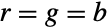
Reduce[Max[r, g, b] - Min[r, g, b] == 0 && 0 ≤ r ≤ 1 && 0 ≤ g ≤ 1 && 0 ≤ b ≤ 1, {r, g, b}, Backsubstitution -> True]Manipulate[ParametricPlot3D[List@@ColorConvert[Hue[h, c / b, b], RGBColor], {h, 0, 1}, {b, 0, 1}, ColorFunction -> Function[{x, y, z}, RGBColor[x, y, z]], Lighting -> "Neutral", Mesh -> None, Axes -> False, PlotLabel -> c, PlotRange -> {0, 1}], {{c, 0.3}, 0, 1}]ISO彩度曲面をISO明度曲面と組み合せて,交点が多面体曲線であることを示す.色相は,白いRGBコーナー( )から分かるように,この多面体曲線周囲の赤から始まる時計回りの長さの比である:
saturation = ParametricPlot3D[List@@ColorConvert[Hue[h, 0.3, b], RGBColor], {h, 0, 1}, {b, 0, 1}, ColorFunction -> Function[{x, y, z}, RGBColor[x, y, z]], Lighting -> "Neutral", Mesh -> None, Axes -> False, PlotRange -> {0, 1}]brightness = ParametricPlot3D[List@@ColorConvert[Hue[h, s, 0.6], RGBColor], {h, 0, 1}, {s, 0, 1}, ColorFunction -> Function[{x, y, z}, RGBColor[x, y, z]], Lighting -> "Neutral", Mesh -> None, Axes -> False, PlotRange -> {0, 1}]ISO色相とISO明度は,彩度曲線(6頂点の多面体曲線)で交差する:
Show[saturation, brightness]特性と関係 (1)
Graphics[Table[{Hue[h], EdgeForm[Gray], Rectangle[{8h, 0}]}, {h, 0, 2, 1 / 8}]]Graphics[Table[{Hue[1 / 4, s], EdgeForm[Gray], Rectangle[{7s, 0}]}, {s, 0, 1, 1 / 7}]]Graphics[Table[{Hue[1 / 4, 1, s], EdgeForm[Gray], Rectangle[{7s, 0}]}, {s, 0, 1, 1 / 7}]]Graphics[Raster[Table[{h, s, 1}, {s, 0, 1, .01}, {h, 0, 1, .01}], ColorFunction -> Hue]]考えられる問題 (1)
Graphics[Table[{Hue[1, s], EdgeForm[Gray], Rectangle[{4s, 0}]}, {s, 0 - 1 / 4, 1 + 1 / 4, 1 / 4}]]Graphics[Table[{Hue[1, 1, b], EdgeForm[Gray], Rectangle[{4b, 0}]}, {b, 0 - 1 / 4, 1 + 1 / 4, 1 / 4}]]プロット関数で,ColorFunctionScalingを使って変数の大域的スケーリングを制御する:
Table[DensityPlot[x, {x, -2, 3}, {y, 0, 1}, FrameTicks -> None, ColorFunction -> (Hue[1, #1]&), ColorFunctionScaling -> t], {t, {False, True}}]おもしろい例題 (3)
Graphics3D[{Opacity[.7], {Hue[#], Cuboid[#, # + .1]}& /@ Tuples[Range[0, 1, .2], 3]}, Axes -> True, AxesLabel -> {"Hue", "Saturation", "Brightness"}, Lighting -> "Neutral"]DynamicModule[{b = .5}, Panel[Row[{Column[{"Lighter", VerticalSlider[Dynamic[b], {0, 1}, ImageSize -> Small], "Darker"}], Graphics[Raster[Table[{h, s, Dynamic[b]}, {s, 0, 1, .05}, {h, 0, 1, .05}], ColorFunction -> Hue]]}]]]Graphics[{Pink, Disk[{100, 100}, 40], Raster[RandomReal[1, {200, 200, 4}], ColorFunction -> Hue]}]
 An Elementary Introduction to the Wolfram Language

 An Elementary Introduction to the Wolfram Language
テキスト
Wolfram Research (1991), Hue, Wolfram言語関数, https://reference.wolfram.com/language/ref/Hue.html (2021年に更新).
CMS
Wolfram Language. 1991. "Hue." Wolfram Language & System Documentation Center. Wolfram Research. Last Modified 2021. https://reference.wolfram.com/language/ref/Hue.html.
APA
Wolfram Language. (1991). Hue. Wolfram Language & System Documentation Center. Retrieved from https://reference.wolfram.com/language/ref/Hue.html