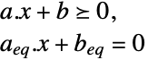
LinearOptimization[c,{a,b}]
求能最小化受线性不等式约束条件 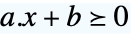 限制的线性目标函数
 的实向量 x.
LinearOptimization[c,{a,b},{aeq,beq}]
包括线性等式约束条件 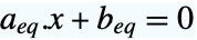 .




LinearOptimization
LinearOptimization[f,cons,vars]
求能最小化受线性约束条件 cons 限制的线性目标函数 f 的变量 vars 的值.
LinearOptimization[c,{a,b}]
求能最小化受线性不等式约束条件 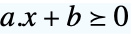 限制的线性目标函数
 的实向量 x.
LinearOptimization[c,{a,b},{aeq,beq}]
包括线性等式约束条件 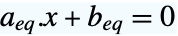 .
LinearOptimization[c,…,{dom1,dom2,…}]
LinearOptimization[…,"prop"]
指定应返回解的 "prop" 属性.
更多信息和选项
- 线性优化也称为线性规划(LP)和混合整数线性规划(MILP).
- 线性优化是凸优化问题,可用实数、整数或复数变量高效地进行全局求解.
- 线性优化求可解决原始问题的
 : »
-
最小化 
受限于约束条件 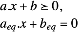
其中 
- 混合整数线性优化给出能求解问题的
 和
 :
-
最小化 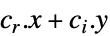
受限于约束条件 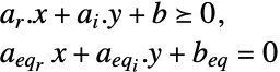
其中 
- 当目标函数取实数值时,LinearOptimization 在内部将
 转换为实变量
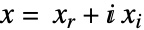 进行求解(其中
 ,
 ).
- 变量指定 vars 应为一个列表,其中的元素以下列形式给出变量:
-
v 名为  的变量,维数由推断而得
v∈Reals 实数标量变量 v∈Integers 整数标量变量 v∈Complexes 复数标量变量 v∈ℛ 限制在几何区域  内的向量变量
v∈Vectors[n,dom]  或
 内的向量变量
v∈Matrices[{m,n},dom]  或
 内的矩阵变量
- 可用以下形式指定约束条件 cons:
-
LessEqual 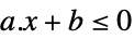
标量不等式 GreaterEqual 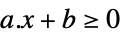
标量不等式 VectorLessEqual 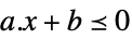
向量不等式 VectorGreaterEqual 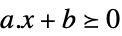
向量不等式 Equal 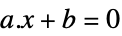
向量或标量等式 Element 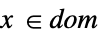
凸域或区域元素 - 对于 LinearOptimization[f,cons,vars],可在约束条件中包括形式为 parval 的参数方程,以定义在 f 或 cons 中使用的参数,其中 par 不在 vars 中,val 是数值或数值数组.
- 原始最小化问题有相关的最大化问题,即拉格朗日对偶问题. 对偶最大值始终小于或等于原始最小值,因此它给出了下限. 对偶最大值点提供了有关原问题的信息,包括最小值对约束条件变化的敏感性.
- 下面给出了线性优化的拉格朗日对偶问题: »
-
最大化 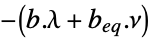
受限于约束条件 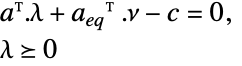
其中 
- 对于线性优化,强对偶性始终成立,这意味着如果原始最小化问题的解存在,那么对偶最大化问题的解也存在,并且对偶最大值等于原始最小值.
- 可能的解的属性 "prop" 包括:
-
"PrimalMinimizer" 
一个最小化目标函数的变量值列表 "PrimalMinimizerRules" 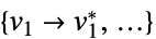
最小化  的变量值 vars={v1,…}
"PrimalMinimizerVector" 
最小化  的向量
"PrimalMinimumValue" 
最小值 
"DualMaximizer" 
最大化 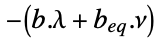 的向量
"DualMaximumValue" 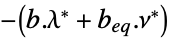
对偶最大值 "DualityGap" 
对偶值和原始最优值之间的差(由于强对偶性,差应为 0) "Slack" 
约束松弛向量 "ConstraintSensitivity" 
 对约束条件扰动的敏感性
"ObjectiveVector" 
线性目标向量 "LinearInequalityConstraints" 
线性不等式约束矩阵和向量 "LinearEqualityConstraints" 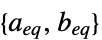
线性等式约束矩阵和向量 {"prop1","prop2",…} 解的几个属性 - 可给出以下选项:
-
MaxIterations Automatic 使用的最大迭代次数 Method Automatic 使用的方法 PerformanceGoal $PerformanceGoal 优化的目标 Tolerance Automatic 内部比较采用的容差 WorkingPrecision Automatic 内部计算使用的精度 - 选项 Method->method 可用来指定使用的方法. 可用的方法包括:
-
Automatic 自动选择方法 "Simplex" 单纯形法 "RevisedSimplex" 修正单纯形法 "InteriorPoint" 内点法(仅适用于机器精度) "CLP" COIN 库线性规划(仅适用于机器精度) "MOSEK" 商业 MOSEK 线性优化求解器 "Gurobi" 商业 Gurobi 线性优化求解器 "Xpress" 商业 Xpress 线性优化求解器 - 当设置为 WorkingPrecision->Automatic 时,精度是从输入参数的精度自动获取的,除非指定的方法仅适用于机器精度,在这种情况下使用机器精度.

范例
打开所有单元 关闭所有单元基本范例 (3)


res = LinearOptimization[x + y, {x + 2y ≥ 3, x ≥ 0, y ≥ 0}, {x, y}]
Show[Plot3D[x + y, {x, 0, 2}, {y, 0, 3}, ...], Graphics3D[{Blue, PointSize[0.04], Point[{x, y, x + y} /. res]}]]

res = LinearOptimization[x + y, {x + 2y == 3, x ≥ 0, y ≥ 0}, {x, y}]LinearOptimization[{1, 1}, {{{1, 0}, {0, 1}}, {0, 0}}, {{{1, 2}}, {-3}}]

LinearOptimization[x + y, {x + 2y == 3, x ≥ 0.5, y ≥ 0}, {x∈Integers, y}]LinearOptimization[{1, 1}, {{{1, 0}, {0, 1}}, {-0.5, 0}}, {{{1, 2}}, {-3}}, {Integers, Reals}]范围 (32)
基本用法 (16)


res = LinearOptimization[x + y, {x + 2y ≥ 3, x ≥ -1, y ≥ -1}, {x, y}]
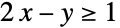

LinearOptimization[x - y, {x + y + z == 1 / 2, x - 2z == 1, 2x - y ≥ 1}, {x, y, z}]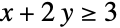


LinearOptimization[x + y, {x + 2y ≥ 3, -1 ≤ x ≤ 2, -1 ≤ y ≤ 1}, {x, y}]用 VectorLessEqual 同时表示几个 LessEqual 不等式约束条件:
LinearOptimization[x + y, VectorLessEqual[{{x - 2y, -x + y}, {3, 2}}], {x, y}]
 以紧凑格式输入向量不等式:
LinearOptimization[x + y, {x - 2y, -x + y}{3, 2}, {x, y}]LinearOptimization[x + y, {x - 2y ≤ 3, -x + y ≤ 2}, {x, y}]用 VectorGreaterEqual 同时表示几个 GreaterEqual 不等式约束条件:
LinearOptimization[x + y, VectorGreaterEqual[{{x + 2y, x}, {3, -1}}], {x, y}]
 以紧凑格式输入向量不等式:
LinearOptimization[x + y, {x + 2y, x}{3, -1}, {x, y}]用 Equal 同时表示几个等式约束条件:
LinearOptimization[x - y, {x + y, x - y} == {1 / 2, 1}, {x, y}]LinearOptimization[x - y, {x + y == 1 / 2, x - y == 1}, {x, y}]LinearOptimization[x + y, {x + 2y ≥ 3, -1{x, y}{2, 1}}, {x, y}]LinearOptimization[x + y, {x + 2y ≥ 3, -1 ≤ x ≤ 2, -1 ≤ y ≤ 1}, {x, y}]

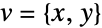
LinearOptimization[{3, 4}.v, {{1, -2}.v ≤ 3, {-1, 1}.v ≤ 2}, v]LinearOptimization[{3, 4}.{x, y}, {{1, -2}.{x, y} ≤ 3, {-1, 1}.{x, y} ≤ 2}, {x, y}]LinearOptimization[{3, 4}.v, {{1, -2}, {-1, 1}}.v{3, 2}, v]

{a, b} = {{{1, 1, 0}, {0, 1, 1}, {1, 1, 1}}, {2, 2, -1}};用 Indexed 指定向量变量的分量,如  :
LinearOptimization[Total[x], {a.xb, Indexed[x, 1] ≥ 1}, x]parameterEqs = {c == {3, 4}, a1 == {1, -2}, a2 == {-1, 1}};
constraints = {a1.{x, y} ≤ 3, a2.{x, y} ≤ 2};LinearOptimization[c.{x, y}, {parameterEqs, constraints}, {x, y}]parameterEqs = {c == {3, 4}, a == {{1, -2}, {-1, 1}}, b == {3, 2}};LinearOptimization[c.{x, y}, {parameterEqs, a.{x, y}b}, {x, y}]LinearOptimization[c.v, {parameterEqs, a.vb}, v]
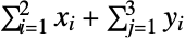
parameterEqs = {a == {{1, 2}, {1, 0}}, b == {3, -1}};LinearOptimization[Total[x] + Total[y], {parameterEqs, a.xb, y1}, {x, y}]
需要的情况下用 Vectors[n] 指定向量变量的维度:
LinearOptimization[Total[x] + Total[y], {parameterEqs, a.xb, y1}, {x, y∈Vectors[3]}]用 NonNegativeReals ( ) 指定非负约束条件:
LinearOptimization[Total[v], {1, 2}.v ≥ 3, v∈Vectors[2, NonNegativeReals]]LinearOptimization[Total[v], {{1, 2}.v ≥ 3, v0}, v]用 NonPositiveReals ( ) 指定非正约束条件:
LinearOptimization[-Total[v], {1, 2}.v-3, v∈Vectors[2, NonPositiveReals]]LinearOptimization[-Total[v], {{1, 2}.v-3, v0}, v]


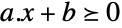

{a, b, c} = {{{1, 2}, {1, 0}, {0, 1}}, {-3, 1, 1}, {1, 1}};LinearOptimization[c, {a, b}]constraints = Thread[a.{x, y} + b ≥ {0, 0, 0}]LinearOptimization[c.{x, y}, constraints, {x, y}]整数变量 (4)
用 Integers 指定整数域约束条件:
LinearOptimization[x - y, N@{x + y + z == 1 / 2, x - 2z == 1, 2x - y ≥ 1}, {x∈Integers, y∈Integers, z}]用 Vectors[n,Integers] 指定向量变量的整数域约束条件:
LinearOptimization[{1., -1}.v, {Total[v] + z == 1 / 2, Indexed[v, 1] - 2z == 1, {2, -1}.v ≥ 1}, {v∈Vectors[2, Integers], z}]用 NonNegativeIntegers ( ) 指定非负整数域约束条件:
LinearOptimization[Total[v], {1, 2}.v ≥ 3., v∈Vectors[2, NonNegativeIntegers]]LinearOptimization[Total[v], {{1, 2}.v ≥ 3., v0}, v∈Vectors[2, Integers]]用 NonPositiveIntegers (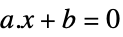 ) 指定非正整数约束条件:
LinearOptimization[-Total[v], {1, 2}.v-3., v∈Vectors[2, NonPositiveIntegers]]LinearOptimization[-Total[v], {{1, 2}.v-3., v0}, v∈Vectors[2, Integers]]复变量 (2)
用 Complexes 指定复变量:
LinearOptimization[Re[z] + Im[z], 1 + 2zI, z∈Complexes]
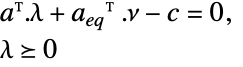
constraints = VectorGreaterEqual[{(-1 + 2I) z, -3}] && VectorGreaterEqual[{z, I}]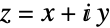
VectorGreaterEqual /@ ComplexExpand[constraints[[All, 1]] /. z -> x + I y]realConstraints = -x - 2y ≥ -3 && 2 x - y ≥ 0 && x ≥ 0 && y ≥ 1;RegionPlot[realConstraints, {x, 0.5, 1}, {y, 1, 1.2}]LinearOptimization[Re[z], constraints, Element[z, Complexes]]LinearOptimization[x, realConstraints, {x, y}]原始模型属性 (3)


LinearOptimization[x + y, {x + 2y >= 3, -1 ≤ x ≤ 2, -1 ≤ y ≤ 1}, {x, y}]LinearOptimization[x + y, {x + 2y >= 3, -1 ≤ x ≤ 2, -1 ≤ y ≤ 1}, {x, y}, "PrimalMinimizer"]LinearOptimization[x + y, {x + 2y >= 3, -1 ≤ x ≤ 2, -1 ≤ y ≤ 1}, {x, y}, "PrimalMinimumValue"]obj = x + y + 1;
cons = {x + 2y ≥ 3, -1 ≤ x ≤ 2, -1 ≤ y ≤ 1};Subscript[p, sym] = LinearOptimization[obj, cons, {x, y}, "PrimalMinimumValue"]{c, {a, b}} = LinearOptimization[obj, cons, {x, y}, {"ObjectiveVector", "LinearInequalityConstraints"}];Subscript[p, m] = LinearOptimization[c, {a, b}, "PrimalMinimumValue"]const = LinearOptimization[obj, cons, {x, y}, "ObjectiveConstant"]Subscript[p, sym] == Subscript[p, m] + constobj = x + y;
cons = {x + 2y == 3, -1 ≤ x ≤ 2, -1 ≤ y ≤ 1};{Subscript[s, ineq], Subscript[s, eq]} = LinearOptimization[obj, cons, {x, y}, "Slack"]{x^ * , {a, b}, {Subscript[a, eq], Subscript[b, eq]}} = LinearOptimization[obj, cons, {x, y}, {...}];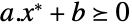


Norm[a.x^ * + b - Subscript[s, ineq]] == 0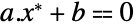


Norm[Subscript[a, eq].x^ * + Subscript[b, eq] - Subscript[s, eq]] == 0
Subscript[s, eq]对偶模型属性 (3)
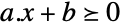


c = {5, 2, 1};
{a, b} = {{{1, 1, 0}, {1, -1, 0}}, {-1, 1}};
{Subscript[a, eq], Subscript[b, eq]} = {{{1, 2, 0}, {1, 1, 1}}, {-3, 2}};
xv = Table[Indexed[x, i], {i, 3}];psol = LinearOptimization[c.xv, {a.xv + b0, Subscript[a, eq].xv + Subscript[b, eq] == 0}, xv]

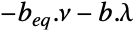
{λv, νv} = {Table[Indexed[λ, i], {i, 2}], Table[Indexed[ν, i], {i, 2}]};dsol = LinearOptimization[b.λv + Subscript[b, eq].νv, {a.λv + Subscript[a, eq].νv == c, λv0}, Join[λv, νv]]{c.xv /. psol, -(b.λv + Subscript[b, eq].νv) /. dsol}
LinearOptimization[c.xv, {a.xv + b0, Subscript[a, eq].xv + Subscript[b, eq] == 0}, xv, "DualityGap"]obj = 5x + 2y + z;
cons = {x + y ≥ 1, x - y ≥ -1, x + 2y == 3, x + y + z == -2};LinearOptimization[obj, cons, {x, y, z}]{c, {a, b}, {Subscript[a, eq], Subscript[b, eq]}} = LinearOptimization[obj, cons, {x, y, z}, {"ObjectiveVector", "LinearInequalityConstraints", "LinearEqualityConstraints"}];

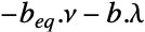
LinearOptimization[b.λ + Subscript[b, eq].ν, {a.λ + Subscript[a, eq].ν == c, λ0}, {λ, ν}]LinearOptimization[5x + 2y + z, {x + y ≥ 1, x - y ≥ -1, x + 2y == 3, x + y + z == -2}, {x, y, z}, "DualMaximumValue"]LinearOptimization[5x + 2y + z, {x + y ≥ 1, x - y ≥ -1, x + 2y == 3, x + y + z == -2}, {x, y, z}, "DualMaximizer"]敏感性属性 (4)
用 "ConstraintSensitivity" 求由约束松弛造成的最优值的变化:
c = {1, -1};
{a, b} = {{{-1, -2}, {-2, -1}, {1, 0}, {0, 1}}, {2., 2., 0, 0}};
p^ * = LinearOptimization[c, {a, b}, "PrimalMinimumValue"];{Subscript[s, λ], Subscript[s, ν]} = LinearOptimization[c, {a, b}, "ConstraintSensitivity"]

δb = {1, 0, 1 / 2, 0};p^ * + δb.Subscript[s, λ]LinearOptimization[c, {a, b + δb}, "PrimalMinimumValue"]{Subscript[s, λ], Subscript[s, ν]} = LinearOptimization[x - y + z, {x + 2y ≤ 2, 2x + y ≤ 2, x ≥ 0, y ≥ 0,
x + y + z == 1}, {x, y, z}, "ConstraintSensitivity"]{{a, b}, {Subscript[a, eq], Subscript[b, eq]}} = LinearOptimization[x - y + z, {x + 2y ≤ 2, 2x + y ≤ 2, x ≥ 0, y ≥ 0, x + y + z == 1}, {x, y, z}, {"LinearInequalityConstraints", "LinearEqualityConstraints"}];Table[{a[[i]].{x, y, z} + b[[i]] ≥ 0, Subscript[s, λ][[i]]}, {i, 4}]Table[{Subscript[a, eq][[i]].{x, y, z} + Subscript[b, eq][[i]] == 0, Subscript[s, ν][[i]]}, {i, 1}]c = {1, -1, 1};
{a, b} = {{{2, -1, 0}, {1, 1, 0}, {0, 1, 0}}, {1, 0, 0}};
{Subscript[a, eq], Subscript[b, eq]} = {{{1, 1, 1}, {1, 0, -2}}, -{1 / 2, 1}};{p^ * , {Subscript[s, λ], Subscript[s, ν]}} = LinearOptimization[c, {a, b}, {Subscript[a, eq], Subscript[b, eq]}, {"PrimalMinimumValue", "ConstraintSensitivity"}]Subscript[s, λ][[2]]p^ * == LinearOptimization[c, {a, b + {0, 1, 0}}, {Subscript[a, eq], Subscript[b, eq]}, "PrimalMinimumValue"]Subscript[s, λ][[1]]p^ * > LinearOptimization[c, {a, b + {1, 0, 0}}, {Subscript[a, eq], Subscript[b, eq]}, "PrimalMinimumValue"]Subscript[s, ν][[1]]p^ * < LinearOptimization[c, {a, b}, {Subscript[a, eq], Subscript[b, eq] + {1, 0}}, "PrimalMinimumValue"]"ConstraintSensitivity" 与问题的对偶最大值点相关:
{{Subscript[s, λ], Subscript[s, ν]}, {λ^ * , ν^ * }} = LinearOptimization[x - y + z, {x + 2y ≤ 2, 2x + y ≤ 2, x ≥ 0, y ≥ 0,
	x + y + z == 1}, {x, y, z}, {"ConstraintSensitivity", "DualMaximizer"}]


Subscript[s, λ] == -λ^ *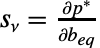


Subscript[s, ν] == -ν^ *选项 (9)
Method (5)
输入为 MachinePrecision 时默认方法是 "CLP":
obj = x + y;
constr = {x + 2 y ≥ 3, -1 ≤ x ≤ 2, -1 ≤ y ≤ 1};LinearOptimization[obj, N[constr], {x, y}, Method -> Automatic]LinearOptimization[obj, N[constr], {x, y}, Method -> "CLP"]任意或无限 WorkingPrecision 情况下的默认方法是 "Simplex":
LinearOptimization[obj, constr, {x, y}, Method -> Automatic]LinearOptimization[obj, constr, {x, y}, Method -> "Simplex"]所有方法都适用于 MachinePrecision 的输入:
obj = x + y;
constr = {x + 2 y ≥ 3, -1 ≤ x ≤ 2, -1 ≤ y ≤ 1};Table[LinearOptimization[obj, N[constr], {x, y}, Method -> met], {met, {"Simplex", "RevisedSimplex", "InteriorPoint", "CLP"}}]"Simplex" 和 "RevisedSimplex" 可被用于任意精度和无限精度的输入:
Table[LinearOptimization[obj, N[constr, 20], {x, y}, Method -> met], {met, {"Simplex", "RevisedSimplex"}}]Table[LinearOptimization[obj, constr, {x, y}, Method -> met], {met, {"Simplex", "RevisedSimplex"}}]a = SparseArray[{Band[{1, 1}] -> 1., Band[{1, 2}] -> 2.}, {500, 300}];"Simplex" 和 "RevisedSimplex" 适用于规模小且密集的问题:
Timing[LinearOptimization[Total[x], {a.x-1, x0}, x, Method -> "Simplex"];]"InteriorPoint" 和 "CLP" 适用于规模大且稀疏的问题:
Timing[LinearOptimization[Total[x], {a.x-1, x0}, x, Method -> "InteriorPoint"];]Timing[LinearOptimization[Total[x], {a.x-1, x0}, x, Method -> "CLP"];]"InteriorPoint" 或 "CLP" 方法可能无法判别问题是不可行的还是无界的:
LinearOptimization[-(x + y), x + y ≥ 1, {x, y}, Method -> "InteriorPoint"]
LinearOptimization[-(x + y), x + y ≥ 1, {x, y}, Method -> "CLP"]
"Simplex" 和 "RevisedSimplex" 可以探测出无界或不可行问题:
LinearOptimization[-(x + y), x + y ≥ 1, {x, y}, Method -> "Simplex"]
如果问题的最优解不是唯一的,不同的方法可能会给出不同的结果:
ContourPlot[-(x + y), {x, y}∈ImplicitRegion[x + y ≤ 1 && x ≥ 0 && y ≥ 0, {x, y}], ContourLabels -> True, ImageSize -> Small]"InteriorPoint" 可能返回最优解集中间位置处的解:
LinearOptimization[-(x + y), {x + y ≤ 1, x ≥ 0, y ≥ 0}, {x, y}, Method -> "InteriorPoint"]LinearOptimization[-(x + y), {x + y ≤ 1, x ≥ 0, y ≥ 0}, {x, y}, Method -> "Simplex"]Tolerance (2)
Tolerance 的设置越小给出的结果越精确:
n = 2000; m = 1000;
Subscript[x, exact] = ConstantArray[1, n];a = SparseArray[{Band[{1, 1}] -> 1, Band[{1, 2}] -> 2}, {m, n}];
b = a.Subscript[x, exact];求使用不同的 Tolerance 设置时计算值和精确最小值  之间的误差:
err = Table[{tol, Abs[n - LinearOptimization[Total[x],
{a.xb, x1}, x, "PrimalMinimumValue", Tolerance -> tol, Method -> "InteriorPoint"]]}, {tol, 10. ^ -Range[7]}]ListLogLogPlot[err, PlotRange -> All, Joined -> True, PlotMarkers -> Automatic]Tolerance 的设置越小给出的答案越精确,但通常情况下要花费更多的时间进行计算:
n = 20000; m = 10000;
a = SparseArray[{Band[{1, 1}] -> 1., Band[{1, 2}] -> 2.}, {m, n}];
b = Range[m];Timing[ptight = LinearOptimization[Total[x] / n, {a.xb, x0}, x, "PrimalMinimumValue", Tolerance -> 10^-12, Method -> "InteriorPoint"];]Timing[ploose = LinearOptimization[Total[x] / n, {a.xb, x0}, x, "PrimalMinimumValue", Tolerance -> 10^-1, Method -> "InteriorPoint"];;]{ptight, ploose}WorkingPrecision (2)
LinearOptimization 根据输入推断要使用的 WorkingPrecision:
LinearOptimization[x + y, {x + 2y ≥ 3, x ≤ 2, y ≤ 1}, {x, y}]MachinePrecision 输入给出 MachinePrecision 输出:
res = LinearOptimization[x + y, {x + 2y ≥ 3., x ≤ 2, y ≤ 1}, {x, y}]Precision[res]LinearOptimization 可使用更高的工作精度计算结果:
LinearOptimization[x + y, {x + 2y ≥ 3, -1 ≤ x ≤ 2, -1 ≤ y ≤ 1}, {x, y}, WorkingPrecision -> 30]LinearOptimization[x + y, {x + 2y ≥ 3.0, -1 ≤ x ≤ 2, -1 ≤ y ≤ 1}, {x, y}, WorkingPrecision -> 30]

应用 (34)
基本模型转换 (8)
最大化受约束条件  限制的
 . 对目标函数取负求解最大化问题:
LinearOptimization[-(x + y), {x + y == 3, x ≥ 0, y ≤ 2}, {x, y}]-LinearOptimization[-(x + y), {x + y == 3, x ≥ 0, y ≤ 2}, {x, y}, "PrimalMinimumValue"]

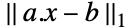
LinearOptimization[Total[s], {a == IconizedObject[«CompoundExpression»], b == Range[10], -sa.x - bs}, {x, s}]

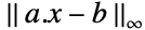
{a, b} = IconizedObject[«CompoundExpression»];LinearOptimization[s, {b - sa.xb + s}, {x, s}]



LinearOptimization[xp + xm, {(xp - xm) + y ≤ 3, (xp - xm) ≥ 1, y ≥ 1, xp ≥ 0, xm ≥ 0}, {xp, xm, y}]
LinearOptimization[t, {x + y ≤ 3, x ≥ 1, y ≥ 1, -t ≤ x ≤ t}, {x, y, t}]


LinearOptimization[x + y, {-1 ≤ 2x + y ≤ 1, x - y ≤ 3}, {x, y}]最小化受约束条件  限制的
 . 约束条件
 可被解释为
 . 根据每个约束条件对问题进行求解:
res1 = LinearOptimization[x + y, {2x + y ≥ 1, x - y ≤ 3, x ≥ 0}, {x, y}, {"PrimalMinimumValue", "PrimalMinimizerRules"}]res2 = LinearOptimization[x + y, {2x + y ≤ -1, x - y ≤ 3, x ≥ 0}, {x, y}, {"PrimalMinimumValue", "PrimalMinimizerRules"}]First@MinimalBy[{res1, res2}, First]Show[Plot3D[x + y, Sequence[...]], Graphics3D[List[...]]]最小化受约束条件  限制的
 ,其中
 是一个非递减函数,因而可代之以最小化
 . 对于两个问题,原始最小点
 将保持不变. 考虑最小化受约束条件
 限制的
 :
f = Function[{s}, s ^ 2];{minval, Subscript[X, min]} = LinearOptimization[x + y, {2x - y ≥ 1, x ≥ 0, y ≥ 0}, {x, y}, {"PrimalMinimumValue", "PrimalMinimizerRules"}]
f[minval]

f = Function[{s}, Exp[s]];

{minval, Subscript[X, min]} = LinearOptimization[(1 + x + 3y), {2x + y ≥ 1, -2 ≤ y ≤ 2, 1 + x + 3y ≥ 0}, {x, y}, {"PrimalMinimumValue", "PrimalMinimizerRules"}]
f[minval]数据拟合问题 (4)
通过最小化  求离散数据的稳健线性拟合. 使用辅助变量
 ,问题被转换为最小化受约束条件
 限制的
 ,这是一个线性优化问题:
{input, output} = IconizedObject[«Block»];
dataplot = ListPlot[output, PlotRange -> All]res = LinearOptimization[Total[s], {a == input, b == output, -sa.x - bs}, {x, s}]Show[ dataplot, Plot[Evaluate[x.{1, t} /. res], {t, 1, 30}]]与用 LeastSquares 获取的拟合进行比较:
line = Fit[output, {1, t}, t]Show[ dataplot, Plot[Evaluate[{x.{1, t} /. res, line}], {t, 1, 30}]]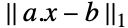
{input, output} = IconizedObject[«Block»];通过添加约束条件 a〚1〛.xb〚1〛,强制曲线穿过第一个数据点:
res = LinearOptimization[Total[s], {a == input, b == output, -sa.x - bs, input[[1]].x == output[[1]]}, {x, s}]Show[Plot[Evaluate[x.{1, t} /. res], {t, 1, 30}, Epilog -> {Red, PointSize[0.02], Point[{1, output[[1]]}]}], ListPlot[output], PlotRange -> All, AxesOrigin -> {0, 0}]通过最小化 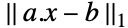 求非线性离散数据的稳健拟合. 生成一些噪音数据:
data = Block[...];
dataPlot = ListPlot[data, PlotRange -> All]

bases = Sqrt[1 + (x - #) ^ 2]& /@ Subdivide[-3, 3, 10];
input = DesignMatrix[data, bases, x, IncludeConstantBasis -> False];
output = data[[All, 2]];res = LinearOptimization[Total[s], {a == input, b == output, -sa.λ - bs}, {λ, s}];Show[dataPlot, Plot[Evaluate[bases.λ /. res], {x, -3, 3}]]lsqfit = Fit[data, bases, x];Plot[{Sin[2x] + Cos[x ^ 2], Evaluate[bases.λ /. res], lsqfit}, {x, -3, 3}, PlotLegends -> {"Reference", "SubscriptBox[L, 1]fit", "Least squares fit"}]通过最小化 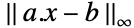 求离散数据的线性拟合. 由于
 ,通过引入标量辅助变量
 ,可将问题转换为最小化受约束条件
 限制的
 :
{a, b} = IconizedObject[«Block»];
dataplot = ListPlot[b, PlotRange -> All]res = LinearOptimization[s, {-s + ba.xs + b}, {x, s}]Show[dataplot, Plot[x.{1, t} /. res, {t, 1, 30}]]可直接用函数 Fit 计算系数:
Fit[b, {1, t}, t, NormFunction -> Infinity]分类问题 (3)



{set1, set2} = IconizedObject[«Block»];
dataPlot = ListPlot[{set1, set2}, PlotMarkers -> {Automatic, PointSize[0.025]}]
对于此分隔问题,第 1 组必须满足 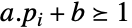 ,第 2 组必须满足
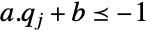 :
res = LinearOptimization[0, {set1.a + b1, set2.a + b-1}, {a, b}]line = a.{x, y} + b /. resShow[RegionPlot[line ≤ 0, {x, 0, 1}, {y, 0, 1}], dataPlot]


{set1, set2} = IconizedObject[«Block»];
dataPlot = ListPlot[{set1, set2}, PlotMarkers -> {Automatic, PointSize[0.025]}]
对于此分隔问题,第 1 组必须满足  ,第 2 组必须满足
 :
poly[{x_, y_}] := {1, x, y, x^2, y^2, x y};
set1Quad = poly /@ set1;
set2Quad = poly /@ set2;res = LinearOptimization[0, {set1Quad.c1, set2Quad.c-1}, c]quad = poly[{x, y}].(c /. res)Show[RegionPlot[quad ≤ 0, {x, -1 / 2, 3 / 2}, {y, -1 / 2, 3 / 2}], dataPlot]set1 = N[{{0, 0}, {-2, -2}, {2, -2}, {2, 2}, {-2, 2}}];
set2 = N[{{0, -1}, {1, 0}, {0, 1}, {-1, 0}}];

pPower[{x_, y_}, {i_, j_}] := If[i == 0, 1, x^i]If[j == 0, 1, y^j];


poly[d_][{x_, y_}] := Sum[Subscript[a, i, j]pPower[{x, y}, {i, j}], {j, 0, d}, {i, 0, d - j}];
variables[d_] := Flatten[Table[Subscript[a, i, j], {j, 0, d}, {i, 0, d - j}]];constraints[d_] := Join[Thread[Map[poly[d], set1] ≤ -1], Thread[Map[poly[d], set2] ≥ 1]];TableForm[constraints[2]]对于此分隔问题,唯一的条件是必须满足所有的约束条件. 将目标向量设置为 0:
d = 0;
maxDegree = 10;
minimizer = Indeterminate;
While[Not[VectorQ[minimizer, NumberQ]],
	If[++d > maxDegree, d = $Failed; Break[]];
	minimizer = Quiet[LinearOptimization[0, constraints[d],
	variables[d], "PrimalMinimizer"]]
	];
drules = LinearOptimization[0, constraints[d], variables[d], "PrimalMinimizerRules"];
separator = poly[d][{x, y}] /. rulesRegionPlot[ImplicitRegion[Evaluate[separator ≤ 0], {x, y}], Epilog -> {PointSize[0.025], Point[set1], Red, Point[set2]}, PlotRange -> {{-3, 3}, {-3, 3}}]生产制造问题 (3)
找到能使公司利润最大化的产品的组合. 公司制造三种产品,下面给出了每个产品制造一件的成本和收入以及最大制造能力:
revenuePerUnit = {90., 100., 70.};
costPerUnit = {45., 40., 20.};
capacity = {100, 40, 60};
每种产品要使用四台机器组合制成,机器在每种产品上花费的时间是:
machineTime = {{20, 10, 10}, {12, 28, 16}, {15, 6, 5}, {10, 15, 0}};Row[BarChart[machineTime[[#]], Sequence[...]]& /@ Range[4]]

profit = (revenuePerUnit - costPerUnit ).xtimeConstraint = machineTime.x2400;capacityConstraint = 0xcapacity;res = LinearOptimization[-profit, {timeConstraint, capacityConstraint}, x]profit /. resGraphicsRow[IconizedObject[«Block»], ImageSize -> 450]同一家公司希望找出改变哪些产品的产能会对利润造成最大的影响. 以前制定的最佳产品组合和利润由下式给出:
timeConstraint = {{20, 10, 10}, {12, 28, 16}, {15, 6, 5}, {10, 15, 0}}.x2400;
capacity = x{100, 40, 60};
profit = {45., 60., 50.}.x;max0 = -LinearOptimization[-profit, {timeConstraint, capacity}, x, "PrimalMinimumValue"]{sens, {a, b}} = LinearOptimization[-profit, {timeConstraint, capacity} , x,
{"ConstraintSensitivity", "LinearInequalityConstraints"}]灵敏度给出了利润相对于每个约束条件的导数. 提取有敏感性的约束条件:
sensPos = Flatten@Position[Chop[sens[[1]]], _ ? (Abs[#] > 0&)]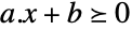
Table[a[[i]].{Subscript[x, 1], Subscript[x, 2], Subscript[x, 3]} + b[[i]] ≥ 0, {i, sensPos}]//TableFormcapacity1 = x{100, 400, 60 + 10};max1 = -LinearOptimization[-profit, {timeConstraint, capacity1} , x, "PrimalMinimumValue"]max1 - max0sens[[1, 7]]×10如果改变产品 1、产品 2 的产能或同时改变两种产品的产能,利润不会增长:
capacity2 = x{100 + 10, 40 + 10, 60};max2 = -LinearOptimization[-profit, {timeConstraint, capacity2}, x, "PrimalMinimumValue"];
max2 - max0找出可以使公司利润最大化的产品组合. 公司制造三种产品  . 每种产品的营收为:
revenuePerUnit = {50., 40., 40.};
laborConstraint = {2, 4, 5}.x ≤ 100;每种产品都包含金和锡. 可用的金和锡的总量分别为 30 和 200 个单位:
goldConstraint = {1, 1, 1}.x ≤ 30;
tinConstraint = {10, 5, 3}.x ≤ 200;setupCost = {500, 500, 300};由于相对较高的设置成本,可能希望根本不生产某些产品. 令  为决策变量,如果生产产品
 ,
 ,否则
 . 限制
 确保如果
 为 0,则
 也为 0,不必对
 作出比其他限制条件更严格的限制:
decisionConstraints = {0w1, 0x1000w};profit = revenuePerUnit.x - setupCost.w;LinearOptimization[-profit, {laborConstraint, goldConstraint,
tinConstraint, decisionConstraints}, {x∈Vectors[3, Integers],
w∈Vectors[3, Integers]}]运输问题 (1)
John Connor 得知 Skynet 计划攻击五个定居点. 他需要将士兵从三个大本营部署到定居点以应对威胁. 将一名士兵从大本营  运送到定居点
 的燃料费用是:
fuelCost = {{10, 15, 15, 10, 20}, {15, 10, 10, 15, 15}, {10, 20, 5, 10, 10}};GraphicsRow[BarChart[fuelCost[[#]], Sequence[...]]& /@ Range[3], Sequence[...]]令  表示从大本营
 运往定居点
 的士兵人数. 要最小化的成本函数是:
totalCost = Total[fuelCost * r, 2];maxSoldiersDeployed = Total[r, {2}]100;minSoldiersNeeded = {Total[r]50, r0};res = LinearOptimization[totalCost, {maxSoldiersDeployed, minSoldiersNeeded}, r∈Matrices[Dimensions[fuelCost]]]TableForm[r /. res, TableHeadings -> {{"Base Camp 1", "Base camp 2", "Base camp 3"}, Array[Subscript[s, #]&, 5]}]最佳分配问题 (2)
Jedi Order 正在与 Dooku 领导的分离主义军队作战. Dooku 和他的两位将军,Asajj Ventress 和 Grievous 将军袭击了三个外围殖民地. Jedi Order 命令三名 Jedi 去帮助外围殖民地. 设  为 Jedi
 击败 Sith
 的几率:
p = {{0.4, 0.5, 0.5}, {0.6, 0.8, 0.6}, {0.7, 0.9, 0.6}};GraphicsRow[BarChart[p[[#]], Sequence[...]]& /@ Range[3], Sequence[...]]设  为矩阵变量,其中如果 Jedi
 与 Sith
 作战,
 为 1,否则为 0. 成本函数为由
 给出的预期的失败次数,用 Inactive[Times] 来构建:
defeats = Total[(1 - p) * x, 2];由于外部殖民地相距很远,每个 Jedi 只能被分配与一个 Sith 作战,反之亦然. 同时,由于  为 0 或 1,则有
 :
constraints = {Total[x] - 1 == 0, Total[x, {2}] - 1 == 0, x0};找出合适的 Jedi 来与 Sith 作战,以尽量减少失败的可能性:
rule = LinearOptimization[defeats, constraints, x∈Matrices[Dimensions[p]]]这意味着 Obi-Wan Kenobi 被派往与 Grievous 将军对战,Mace Windu 被派往与 Asajj Ventress 对战,Ki-Adi-Mundi 则与 Dooku 对战. 预期的失败次数是:
LinearOptimization[defeats, constraints, x∈Matrices[Dimensions[p]], "PrimalMinimumValue"]

weights = IconizedObject[«Block»];设  为矩阵变量,其中,当
 与
 匹配时,
 为 1,否则为 0. 匹配的总权重由
 给出,用 Inactive[Times] 来构建:
cost = Total[weights * x, 2];

constraints = {Total[x] == 1, Total[x, {2}] == 1, x0};用 LinearOptimization 求解问题:
{minCost, rule} = LinearOptimization[cost, constraints, x∈Matrices[Dimensions[weights]], {"PrimalMinimumValue", "PrimalMinimizerRules"}]可以通过将矩阵  转换为图来提取匹配置换. Round 用于对由某些方法中的数值错误引起的较小的值进行截断:
graph = AdjacencyGraph[Round[x /. rule]];edges = EdgeList[graph] /. DirectedEdge[i_, j_] :> DirectedEdge[Subscript[a, i], Subscript[b, j]];
Graph[edges, Sequence[...]]库存控制问题 (2)
求为最小化成本零售店每周必须为产品  订购的库存. 设
 为第
 周开始时可用的库存,
 为第
 周开始时批发商收到的订单. 从批发商处购买一件产品的成本是 $3:
purchaseCost = 3u;
purchaseConstraint = u0;持有多余或负库存的成本为每件产品 $1. 库存成本为  ,它不是线性的,但可用
 来表示:
inventoryCost = xp + xm;
inventoryConstraints = {xp0, xm0};
totalCost = Total[inventoryCost + purchaseCost];设  为第
 周开始时的需求. 52 周的总需求为
 ,
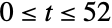 . 商店的库存按
 演化:
n = 52;
w = 6. + 5Sin[Subdivide[0, 2Pi, n]];
a = SparseArray[{Band[{1, 1}] -> -1., Band[{1, 2}] -> 1.}, {n + 1, n + 1}];
demandConstraint = a.(xp - xm) == Inactive[Plus][u, -w];
在第 0 周,持有的库存为  ,订单为
 . 商店每周向批发商订购的数量不得超过 10 件:
initialInventory = {Indexed[xp, 1] - Indexed[xm, 1] == 10, Indexed[u, 1] == 5};
maxOrder = u10;通过最小化成本求商店应持有的最佳库存和应向批发商订购的数量:
vars = Element[#, Vectors[n + 1, Reals]]& /@ {xp, xm, u};
res = LinearOptimization[totalCost, {purchaseConstraint, inventoryConstraints, demandConstraint, initialInventory, maxOrder}, vars];
下面是库存、订单和需求的绘图,显示在第 26 周之后,商店不需要任何库存,因此最大限度地降低了库存成本:
ListLinePlot[{xp - xm, u, w} /. res, PlotRange -> All, PlotStyle -> {Red, Blue, Green}, PlotLegends -> {"Inventory", "Stock order", "Demand"}]求零售店每周必须为产品  订购的库存,在不出现延期交货的情况下最小化成本. 设
 为第
 周开始时批发商收到的订单. 从批发商处购买一件产品的成本是 $3:
purchaseCost = 3u;
purchaseConstraint = u0;inventoryCost = xp + xm;
inventoryConstraints = {xp0, xm0};设  为第
 周开始时的需求. 52 周的总需求为
 ,
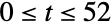 . 商店的库存按
 演化:
n = 52;
w = 6. + 5Sin[Subdivide[0, 2Pi, n]];
a = SparseArray[{Band[{1, 1}] -> -1., Band[{1, 2}] -> 1.}, {n + 1, n + 1}];
demandConstraint = a.(xp - xm) == Inactive[Plus][u, -w];
开始时的库存为  、
 ,商店一次向批发商订购的最大数量为 10 件:
initialInventory = {Indexed[xp, 1] - Indexed[xm, 1] == 10, Indexed[u, 1] == 5};
maxOrder = u0;
noBackOrders = xp - xm0;通过最小化成本求商店应持有的最佳库存和应向批发商订购的数量:
vars = Element[#, Vectors[n + 1, Reals]]& /@ {xp, xm, u};
res = LinearOptimization[Total[purchaseCost + inventoryCost], {purchaseConstraint, inventoryConstraints, demandConstraint, initialInventory, maxOrder, noBackOrders}, vars];
下面的绘图显示为避免出现延期交货的情况,必须在开始的几周购买多余的产品以满足需求. 商店从第 20 周到第 21 周期间开始没有库存费用:
ListLinePlot[{xp - xm, u, w} /. res, PlotRange -> All, PlotStyle -> {Red, Blue, Green}, PlotLegends -> {"Inventory", "Stock order", "Demand"}]结构优化问题 (2)
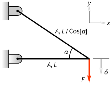
重量为  ,其中
 为密度,
 和
 为杆件 1 和 杆件 2 的横截面面积. 此处假定
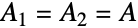 :
weight = ρ A l(1 / Cos[α] + 1);{Subscript[F, 1], Subscript[F, 2]} = {F / Sin[α], F / Tan[α]};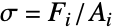


forceConstraints = {Subscript[F, 1] ≤ A Subscript[σ, max], Subscript[F, 2] ≤ A Subscript[σ, max]};自由节点处的位移为  . 此位移沿杆件的轴的分量必须等于位移
 ,其中
 为杨氏模量:
deqns = {(Subscript[F, 1]l / Cos[α]) / (Y A) == Subscript[δ, x] / Cos[α] + Subscript[δ, y] / Sin[α], (Subscript[F, 2] l) / (Y A) == Subscript[δ, x]};
displacementConstraint = A(Subscript[δ, y] /. First@Solve[deqns, {Subscript[δ, x], Subscript[δ, y]}]) ≤ δ A;params = {Y -> 69 10^6, ρ -> 2700., Subscript[σ, max] -> 69000, α -> Pi / 6, l -> 1, F -> 10^3, δ -> 10^-2};LinearOptimization[weight /. params, {forceConstraints, displacementConstraint} /. params, A, {"PrimalMinimumValue", "PrimalMinimizerRules"}]minTrussWeight[α_ ? NumericQ, l_ ? NumericQ] := Module[{A}, LinearOptimization[Sequence[...], A, "PrimalMinimumValue"]];ContourPlot[minTrussWeight[x, y], Sequence[...]]最小化受到压迫力和位移约束的双梁桁架的重量,并找到对桁架设计有重大影响的约束条件:
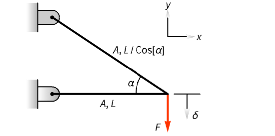
重量为  ,其中
 为密度,
 和
 为杆件 1 和 杆件 2 的横截面面积. 此处假定
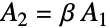 :
weight = ρ A l(1 / Cos[α] + β);{Subscript[F, 1], Subscript[F, 2]} = {F / Sin[α], F / Tan[α]};
forceConstraints = {A Subscript[σ, max] - Subscript[F, 1] ≥ 0, A β Subscript[σ, max] - Subscript[F, 2] ≥ 0};
displacementConstraint = δ A β Y - F l(β Sec[α] - 1) ≥ 0;params = {Y -> 69 10^6, ρ -> 2700., Subscript[σ, max] -> 69000, α -> Pi / 6, l -> 1, F -> 10^3, δ -> 10^-2, β -> 1.1};
LinearOptimization[weight /. params, {forceConstraints, displacementConstraint} /. params, A, {"PrimalMinimumValue", "PrimalMinimizerRules"}]{sens, {a, b}} = LinearOptimization[weight /. params, {forceConstraints, displacementConstraint} /. params, A, {"ConstraintSensitivity", "LinearInequalityConstraints"}];
senssi = First@Flatten@Position[Chop[sens[[1]]], x_ /; Abs[x] > 0]影响设计的关键约束条件是作用于杆件 1 上的力的约束条件 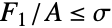 :
{a[[si]].{A} + b[[si]] ≥ 0, forceConstraints[[1]] /. params}顺序线性优化 (1)
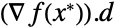
最小化受非线性约束条件  限制的非线性函数
 . 可将
 近似为
 ,将约束条件
 近似为
 . 这样我们就得到了一个可以迭代求解的线性最小化问题. 考虑下面这种情况,其中
 ,
 :
f[{x_, y_}] := -x^2 Exp[-y^2];
g[{x_, y_}] := {25 - x^2 - y^2, 12 - x - 2y, x, y};df[{x_, y_}] = D[f[{x, y}], {{x, y}}];
dg[{x_, y_}] = D[g[{x, y}], {{x, y}}];

LinearSubProblem[xiter_] := Module[{c, a, b},
	{c, a, b} = #[xiter]& /@ {df, dg, g};
	LinearOptimization[c, {a, b}]
	];
从初始猜测 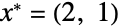 开始进行迭代. 下一步为
 ,其中
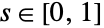 是确保始终满足约束条件的步长:
x^ *  = {2., 1.};
xp = Last@Reap[Do[
	Sow[x^ * , "IterationPoints"];
	d = LinearSubProblem[x^ * ];
	If[Norm[d] ≤ 10 ^ -5, Break[]];
	s = 1;
	While[Min[g[x^ *  + s * d]] ≤ 0, s /= 2];
	x^ *  += s * d;
, {20}], "IterationPoints"]ContourPlot[f[{x, y}], {x, 0, 6}, {y, 0, 2}, Sequence[...]]数独游戏 (3)
sudokuDisplay[board_ ? MatrixQ] := Module[...];
sudokuDisplay[known = SparseArray[{...}, {9, 9}, _]]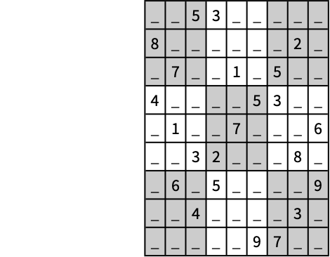
设  为子方格
 的变量. 设
 为向量
 的元素
 .
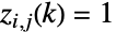 时,
 中的数字为
 . 每个
 只含有一个数字,所以
 只能含有一个非零元素,即
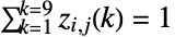 :
squareConstraints = Table[{Total[z[i, j]] == 1, 0z[i, j]1,
z[i, j]∈Vectors[9, Integers]}, {i, 9}, {j, 9}];

onesVector = ConstantArray[1, 9];
rowConstraints = Table[Sum[z[i, j], {j, 9}] == onesVector, {i, 9}];
columnConstraints = Table[Sum[z[i, j], {i, 9}] == onesVector, {j, 9}];
blockConstraints = Table[Sum[z[i + m, j + n], {m, 3}, {n, 3}] == onesVector, {i, {0, 3, 6}}, {j, {0, 3, 6}}];sudokuConstraints = {squareConstraints, rowConstraints, columnConstraints, blockConstraints};vars = Flatten[Table[z[i, j], {i, 9}, {j, 9}]];

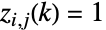
knownConstraints = MapThread[Indexed[z@@#1, #2] == 1&, {known["NonzeroPositions"], known["NonzeroValues"]}];res = LinearOptimization[0, {sudokuConstraints, knownConstraints}, vars];sudokuDisplay[SparseArray@MapThread[List@@#1 -> Range[9].#2&,
{vars, vars /. res}]]通过随机指定第一行来生成随机数独板. 根据上述过程定义一个求解器函数:
sudokuSolve[known_SparseArray] := Module[...];
sudokuDisplay[board_ ? MatrixQ] := Module[...];known = SparseArray[Thread[{1, Range[9]}] -> RandomSample[Range[9]], {9, 9}, _];sudokuDisplay /@ {sudokuSolve[known], known}随机生成一个题板,并一次删除一个元素以生成数独谜题. 定义解决数独难题的函数. 如果在数独题板上指定了负数,则该函数假定不允许在该位置上出现这样的数字:
sudokuSolve[known_SparseArray] := Module[...];
sudokuDisplay[board_ ? MatrixQ] := Module[...];known = SparseArray[Thread[{1, Range[9]}] -> RandomSample[Range[9]], {9, 9}];
refSudokuMat = sudokuSolve[known]minElementsToKeep = 30;一次从题板上删除一个随机选择的元素,重复进行,直到为了保持解的唯一性不能再删除更多元素. 通过解数独难题来测试删除,条件是删除的元素不能取删除的数字. 如果找到可行的解,则该位置上的数字不是唯一的,将保留该元素;否则,将其从题板上移除:
sudokuElements = RandomSample[Thread[
	refSudokuMat["NonzeroPositions"] -> refSudokuMat["NonzeroValues"]]];
n = 81;i = 1;
While[Length[sudokuElements] > minElementsToKeep  && i < n,
	newElements = sudokuElements;
	newElements[[i, 2]] *= -1; (* Specify the element as negative number *)
	res = sudokuSolve[SparseArray[newElements, {9, 9}]];
	If[res === $Failed, sudokuElements = Delete[sudokuElements, i];n--, i++];
];sudokuDisplay[sudokuPuzzle = SparseArray[sudokuElements, {9, 9}, _]]sudokuDisplay /@ {sudokuSolve[sudokuPuzzle], refSudokuMat}图的着色问题 (1)
求为图的节点着色所需的最小颜色数量,以使两个相邻节点的颜色不同. 从足够多的颜色开始:
nColors = 6;SeedRandom[123];
nNodes = 100;
graph = RandomGraph[DegreeGraphDistribution[Table[3, nNodes]], VertexSize -> {"Scaled", 0.02}];提取与图关联的邻接矩阵. 由于矩阵是对称的,因此仅使用矩阵的上三角部分:
graphMat = UpperTriangularize[AdjacencyMatrix[graph]];设  为一个矩阵,如果为节点
 分配了颜色
 ,则
 . 令
 为一个向量,如果最后使用了颜色
 ,则
 . 必须为每个节点分配一个颜色:
nodeConstraint = Total[x, {2}] == 1;sameColorConstraint = Table[{i, j} = ci;Table[Indexed[x, {i, k}] + Indexed[x, {j, k}] ≤ 1, {k, nColors}], {ci, graphMat["NonzeroPositions"]}];


colorConstraint = Table[Indexed[x, {i, k}] ≤ Indexed[y, k], {i, nNodes}, {k, nColors}];

binaryConstraint = {0x1, 0y1};res = LinearOptimization[Total[y], {nodeConstraint, sameColorConstraint,
colorConstraint, binaryConstraint}, {x∈Matrices[{nNodes, nColors}, Integers], y∈Vectors[nColors, Integers]}];Total[y] /. rescolors = {Red, Green, Blue, Brown, Yellow, Magenta};
HighlightGraph[graph, SparseArray[x /. res]["NonzeroPositions"] /. {i_, j_} :> Style[i, colors[[j]]]]集合覆盖问题 (3)
求医院急诊室必须待命的医生的最佳组合,以便急诊室可以完成一系列手术. 每位医生只能完成一定数量的手术:
TableForm[procedureChart = (| | | | | | |
| - | - | - | - | - | - |
| 1 | 0 | 0 | 1 | 0 | 0 |
| 1 | 0 | 0 | 0 | 1 | 0 |
| 0 | 1 | 1 | 0 | 0 | 0 |
| 1 | 0 | 0 | 0 | 0 | 1 |
| 0 | 1 | 1 | 0 | 0 | 1 |
| 0 | 1 | 0 | 1 | 0 | 0 |), Rule[...]]cost = {3000, 4000, 2000, 2000, 1000, 2000};


objective = cost.x;
procedureConstraint = procedureChart.x1;LinearOptimization[objective, {procedureConstraint, 0x1.}, x∈Vectors[6, Integers]]给出一个包含六个区的城市必须建立的最佳消防站数量,以使每个区 15 分钟之内至少有一个消防站. 在各区之间行驶所需的时间为:
TableForm[dist = (| | | | | | |
| -- | -- | -- | -- | -- | -- |
| 0 | 10 | 20 | 30 | 30 | 20 |
| 10 | 0 | 25 | 35 | 20 | 10 |
| 20 | 25 | 0 | 15 | 30 | 20 |
| 30 | 35 | 15 | 0 | 15 | 25 |
| 20 | 20 | 30 | 15 | 0 | 14 |
| 20 | 10 | 20 | 25 | 14 | 0 |), Rule[...]]令  为决策变量,如果在城区
 建消防站则
 . 目标是最小化消防站的数量:
objective = Total[x];decisionMatrix = N@Table[If[dist[[i, j]] ≤ 15, 1, 0], {i, 6}, {j, 6}];
stationConstraint = decisionMatrix.x 1;LinearOptimization[objective, {stationConstraint, 0x1}, x∈Vectors[6, Integers]]求公司需要建立的最少数量的配送仓库,以便为六个零售商店配送货物. 该公司选择了五个可能的地点. 每个仓库为每个商店配送货物的成本为:
TableForm[transportCost = (| | | | | | |
| -- | -- | -- | -- | -- | -- |
| 10 | 15 | 8 | 11 | 10 | 12 |
| 15 | 12 | 11 | 11 | 10 | 10 |
| 12 | 10 | 11 | 12 | 8 | 15 |
| 10 | 8 | 15 | 11 | 12 | 12 |
| 15 | 12 | 12 | 10 | 15 | 8 |), Rule[...]]overheadCost = {12, 12, 12, 12, 10};令  为决策变量,如果要建造仓库
 则
 . 令
 表示仓库
 提供给商店
 的商品份额. 目标是最小化成本:
objective = Total[Inactive[Times][transportCost, x], 2] + overheadCost.y;
goodsConstraint = {Total[x] == 1, x0};depotConstraint = Table[Indexed[x, {i, j}] ≤ Indexed[y, i], {i, 5}, {j, 6}];res = LinearOptimization[N@objective, {depotConstraint, goodsConstraint,
0y1}, {x∈Matrices[{5, 6}], y∈Vectors[5, Integers]}]Flatten@Position[y /. res, 1]旅行商问题 (1)
找到一条推销员应选的穿过  个城市的路径,只访问每个城市一次,最小化行走的距离. 生成位置:
n = 20;
pts = CompoundExpression[...];
令  为城市
 和城市
 之间的距离. 令
 为决策变量,如果
 ,则路径从城市
 到城市
 ,目标是最小化距离:
c = DistanceMatrix[pts, pts];
objective = Total[Inactive[Times][c, x], 2];travelConstraint = {Total[x] == 1, Total[x, {2}] == 1};cityConstraint = Table[Indexed[x, {i, i}] == 0, {i, n}];singleTourConstraint = Flatten[Table[If[i == j, {},
Indexed[u, i] - Indexed[u, j] + n * Indexed[x, {i, j}] ≤ n - 1], {i, 2, n}, {j, 2, n}]];
variableConstraint = {0x1, 0un - 1};res = LinearOptimization[objective, {travelConstraint, cityConstraint,
singleTourConstraint, variableConstraint}, {u∈Vectors[n],
x∈Matrices[{n, n}, Integers]}] ;
Short[res, 2]FindCycle[AdjacencyGraph[x /. res], {n}][[1]]Activate[objective /. res]用 FindShortestTour 来求解旅行商问题要更高效:
FindShortestTour[pts]属性和关系 (9)
LinearOptimization 给出目标函数的全局最小值:
res = LinearOptimization[x + 2y, {3x + 4y ≥ 5, x ≥ 0, y ≥ 0}, {x, y}]Show[Plot3D[x + 2y, {x, y}∈ImplicitRegion[3x + 4y ≥ 5 && x ≥ 0 && y ≥ 0, {x, y}]], Graphics3D[{PointSize[0.05], Point[{x, y, x + 2y} /. res]}]]Minimize 也可给出线性优化问题的全局精确结果:
Minimize[{x + 2y, {3x + 4y ≥ 5 && x ≥ 0 && y ≥ 0}}, {x, y}]NMinimize 可用全局方法获得近似结果:
NMinimize[{x + 2y, {3x + 4y ≥ 5 && x ≥ 0 && y ≥ 0}}, {x, y}]FindMinimum 可用局部方法获得近似结果:
FindMinimum[{x + 2y, {3x + 4y ≥ 5 && x ≥ 0 && y ≥ 0}}, {x, y}]LinearFractionalOptimization 用 LinearOptimization 来求解问题:
LinearFractionalOptimization[(Subscript[x, 1] + Subscript[x, 2]) / (1 + 3Subscript[x, 1] + 2Subscript[x, 2]), {Subscript[x, 1] + Subscript[x, 2] ≥ 2, Subscript[x, 1] ≥ 0, Subscript[x, 2] ≥ 0}, {Subscript[x, 1], Subscript[x, 2]}]
obj = (Subscript[y, 1] + Subscript[y, 2]);
constraints = {Subscript[y, 1] + Subscript[y, 2] - 2t ≥ 0, Subscript[y, 1] ≥ 0, Subscript[y, 2] ≥ 0, t ≥ 0, 3Subscript[y, 1] + 2Subscript[y, 2] + t == 1};res = LinearOptimization[obj, constraints, {Subscript[y, 1], Subscript[y, 2], t}]{Subscript[y, 1] / t, Subscript[y, 2] / t} /. resQuadraticOptimization 是 LinearOptimization 的推广:
LinearOptimization[x + 2y, {3x + 4y ≥ 5, x ≥ 0, y ≥ 0}, {x, y}]QuadraticOptimization[x + 2y, {3x + 4y ≥ 5, x ≥ 0, y ≥ 0}, {x, y}]SecondOrderConeOptimization 是 LinearOptimization 的推广:
LinearOptimization[x + 2y, {3x + 4y ≥ 5, x ≥ 0, y ≥ 0}, {x, y}]SecondOrderConeOptimization[x + 2y, {3x + 4y ≥ 5, x ≥ 0, y ≥ 0}, {x, y}]SemidefiniteOptimization 是 LinearOptimization 的推广:
LinearOptimization[x + 2y, {3x + 4y ≥ 5, x ≥ 0, y ≥ 0}, {x, y}]SemidefiniteOptimization[x + 2y, {3x + 4y ≥ 5, x ≥ 0, y ≥ 0}, {x, y}]ConicOptimization 是 LinearOptimization 的推广:
LinearOptimization[x + 2y, {3x + 4y ≥ 5, x ≥ 0, y ≥ 0}, {x, y}]ConicOptimization[x + 2y, {3x + 4y ≥ 5, x ≥ 0, y ≥ 0}, {x, y}]可能存在的问题 (6)
res = LinearOptimization[x + y, {x - 2y ≤ 3, x > 1, y > 0}, {x, y}]原因是 LinearOptimization 求解的是  :
{x - 2y ≤ 3, x > 1, y > 0} /. res
LinearOptimization[x, {x ≤ 0, x ≥ 1}, x, "PrimalMinimumValue"]
最小点为 Indeterminate:
LinearOptimization[x, {x ≤ 0, x ≥ 1}, x]

LinearOptimization[-(x + y), x + y ≥ 1, {x, y}, "PrimalMinimumValue"]
最小点为 Indeterminate:
LinearOptimization[-(x + y), x + y ≥ 1, {x, y}]
LinearOptimization[x + y, {x + y == 2.1, 1 ≤ y ≤ 2}, {x∈Integers, y}, {"DualMaximumValue", "DualMaximizer", "DualityGap"}]LinearOptimization[x + y, {x + y == 21 / 10, 1 ≤ y ≤ 2}, {x∈Integers, y}]
LinearOptimization[Re[z] + Im[z], 1 + 2zI, z∈Complexes]只使用 GreaterEqual 是不可行的:
LinearOptimization[Re[z] + Im[z], 1 + 2z ≥ I, z∈Complexes]

文本
Wolfram Research (2019),LinearOptimization,Wolfram 语言函数,https://reference.wolfram.com/language/ref/LinearOptimization.html (更新于 2020 年).
CMS
Wolfram 语言. 2019. "LinearOptimization." Wolfram 语言与系统参考资料中心. Wolfram Research. 最新版本 2020. https://reference.wolfram.com/language/ref/LinearOptimization.html.
APA
Wolfram 语言. (2019). LinearOptimization. Wolfram 语言与系统参考资料中心. 追溯自 https://reference.wolfram.com/language/ref/LinearOptimization.html 年