


MomentOfInertia
MomentOfInertia[reg,pt,v]
计算围绕过 pt 点沿 v 方向的轴转动的区域 reg 的转动惯量.
MomentOfInertia[reg]
计算区域 reg 对质心的转动惯量矩阵.
MomentOfInertia[reg,pt]
计算相对点 pt 的转动惯量矩阵.
更多信息和选项
- 转动惯量惯又叫做质量惯性矩或惯量矩. 转动惯量惯矩阵又叫做质量惯性矩矩阵或惯量矩矩阵.
- 转动惯量是刚体对转动加速度的抵抗. 它在转动运动中的作用类似于平动中的质量. 质量是对平动加速度的抵抗.
-
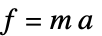
平动加速度 力  , 加速度
 , 质量


转动加速度 力矩  , 转动加速度
 , 转动惯量

- MomentOfInertia[reg,pt] 给出关于点 pt 的转动惯量,并由下式得到:
-
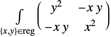
二维转动惯量矩阵 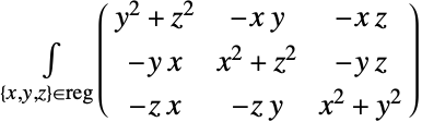
三维转动惯量矩阵 - 其中 reg 由区域 reg 平移 -pt 得到.
- 转动惯量矩阵 ℐ 通过公式
 可用来计算沿任何方向 v 的转动惯量. 在二维情况下,v 必须在
 -
 平面内. »
- MomentOfInertia 是假定区域的质量密度为常数的情况下给出计算结果.
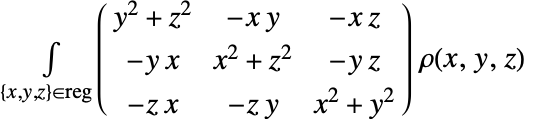
- 对于变质量密度
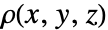 , 要按照以下公式用 Integrate 或 NIntegrate 计算出转动惯量矩阵. »
-
范例
打开所有单元 关闭所有单元基本范例 (4)


MomentOfInertia[Ball[], {1, 1, 0}, {0, 0, 1}]Graphics3D[{Ball[], Thick, InfiniteLine[{1, 1, 0}, {0, 0, 1}]}]ℐ = MomentOfInertia[Ball[], {1, 1, 0}]运用这个矩阵和一个归一化的向量,可以求出围绕任何轴的转动惯量:
{0, 0, 1}.ℐ.{0, 0, 1}MomentOfInertia[Ball[]]这相当于通过 RegionCentroid 来指定中心点:
MomentOfInertia[Ball[], RegionCentroid[Ball[]]]MomentOfInertia[Ball[{0, 0, 0}, r], {0, 0, 0}, {1, 1, 1}]范围 (26)
特殊区域 (15)
长  ,宽
 的 Rectangle:
reg = Rectangle[{-l / 2, -w / 2}, {l / 2, w / 2}];
MomentOfInertia[reg, Assumptions -> l > 0 && w > 0]//MatrixFormRegion[reg /. {l -> 3, w -> 2}]半径为  的 Disk:
reg = Disk[{0, 0}, r];
MomentOfInertia[reg, Assumptions -> r > 0]//MatrixFormRegion[reg /. {r -> 1}]

reg = Disk[{0, 0}, {a, b}];
MomentOfInertia[reg, Assumptions -> a > 0 && b > 0]//MatrixFormRegion[reg /. {a -> 3, b -> 2}]半径为  和
 的 Annulus:
reg = Annulus[{0, 0}, {Subscript[r, 1], Subscript[r, 2]}];
MomentOfInertia[reg, Assumptions -> Subscript[r, 2] > Subscript[r, 1] > 0]//MatrixFormRegion[reg /. {Subscript[r, 1] -> 1, Subscript[r, 2] -> 2}]长为  ,半径为
 的 StadiumShape:
reg = StadiumShape[{{-l / 2, 0}, {l / 2, 0}}, r];
MomentOfInertia[reg, Assumptions -> l > 0 && r > 0]//MatrixFormRegion[reg /. {r -> 1, l -> 2}] 边长为  和
 的正 Triangle:
reg = Triangle[{{0, 0}, {a, 0}, {0, b}}];
MomentOfInertia[reg, Assumptions -> a > 0 && b > 0]//MatrixFormRegion[reg /. {a -> 4, b -> 3}]长为  ,宽为
 ,高为
 的 Cuboid:
body = Cuboid[{-l / 2, -w / 2, -h / 2}, {l / 2, w / 2, h / 2}];
MomentOfInertia[body, Assumptions -> l > 0 && w > 0 && h > 0]//MatrixFormRegion[body /. {l -> 3, w -> 2, h -> 1}]半径为  的 Ball:
body = Ball[{0, 0, 0}, r];
MomentOfInertia[body, Assumptions -> r > 0]//MatrixFormRegion[body /. {r -> 1}]半轴为  ,
 和
 的 Ellipsoid:
body = Ellipsoid[{0, 0, 0}, {a, b, c}];
MomentOfInertia[body, Assumptions -> a > 0 && b > 0 && c > 0]//MatrixFormRegion[body /. {a -> 5, b -> 4, c -> 3}]半径为  和
 的 SphericalShell:
body = SphericalShell[{0, 0, 0}, {Subscript[r, 1], Subscript[r, 2]}];
MomentOfInertia[body, Assumptions -> Subscript[r, 2] > Subscript[r, 1] > 0]//MatrixFormGraphics3D[{Opacity[0.7], body /. {Subscript[r, 1] -> 1, Subscript[r, 2] -> 2}}]长为  ,半径为
 的 Cylinder:
body = Cylinder[{{-l / 2, 0, 0}, {l / 2, 0, 0}}, r];
MomentOfInertia[body, Assumptions -> l > 0 && r > 0]//MatrixFormRegion[body /. {r -> 1, l -> 2}]长为  ,半径为
 的 CapsuleShape:
body = CapsuleShape[{{-l / 2, 0, 0}, {l / 2, 0, 0}}, r];
MomentOfInertia[body, Assumptions -> l > 0 && r > 0]//MatrixFormRegion[body /. {r -> 1, l -> 2}]边长为  ,
 和
 的长方形 Tetrahedron:
body = Tetrahedron[{{0, 0, 0}, {a, 0, 0}, {0, b, 0}, {0, 0, c}}];
MomentOfInertia[body, Assumptions -> a > 0 && b > 0 && c > 0]//MatrixFormRegion[body /. {a -> 5, b -> 4, c -> 3}]边长为  和
 ,高为
 的长方形 Pyramid:
body = Pyramid[{{-a / 2, -b / 2, 0}, {a / 2, -b / 2, 0}, {a / 2, b / 2, 0}, {-a / 2, b / 2, 0}, {0, 0, h}}];
MomentOfInertia[body, Assumptions -> a > 0 && b > 0 && h > 0]//MatrixFormRegion[body /. {a -> 5, b -> 4, h -> 3}]边长为  和
 ,高为
 的长方形 Prism:
body = Prism[{{0, -b / 2, h}, {-a / 2, -b / 2, 0}, {a / 2, -b / 2, 0}, {0, b / 2, h}, {-a / 2, b / 2, 0}, {a / 2, b / 2, 0}}];
MomentOfInertia[body, Assumptions -> a > 0 && b > 0 && h > 0]//MatrixFormRegion[body /. {a -> 5, b -> 4, h -> 3}]公式确定的区域 (2)
表示为一个 ImplicitRegion 的圆盘的惯量矩阵:
MomentOfInertia[ImplicitRegion[x^2 + y^2 ≤ 1, {x, y}]]MomentOfInertia[ImplicitRegion[x^2 + y^2 ≤ 1, {x, y, {z, 0, 2}}], {1, 1, 1}, {1, 1, 1}]表示为一个 ParametricRegion 的圆盘的转动惯量:
MomentOfInertia[ParametricRegion[{r Cos[θ], r Sin[θ]}, {{r, 0, 1}, {θ, 0, 2π}}], {1, 1}, {1, 2}]MomentOfInertia[ParametricRegion[{r(1 - t^2/1 + t^2), r(2t/1 + t^2)}, {t, {r, 0, 1}}], {1, 1}, {1, 2}]MomentOfInertia[ParametricRegion[{r Cos[θ], r Sin[θ], z}, {{r, 0, 1}, {θ, 0, 2π}, {z, 0, 2}}], {1, 1, 1}, {1, 2, 3}]网格区域 (2)
二维情况下一个 MeshRegion 的转动惯量矩阵:
reg = DelaunayMesh[RandomReal[1, {10, 2}]]MomentOfInertia[reg]reg = MeshRegion[{{0, 0}, {1, 0}, {2, -1}, {2, 1}}, {Line[{{1, 2, 3, 4, 2}}]}]MomentOfInertia[reg]reg = DelaunayMesh[RandomReal[1, {20, 3}]]MomentOfInertia[reg]MomentOfInertia[reg, {1, 0, 1}]一个 BoundaryMeshRegion 的转动惯量矩阵:
reg = ConvexHullMesh[RandomReal[1, {10, 2}]]MomentOfInertia[reg]reg = ConvexHullMesh[RandomReal[1, {30, 3}]]MomentOfInertia[reg]导出区域 (3)
一个 RegionIntersection 的转动惯量:
reg = RegionIntersection[Disk[{0, 0}, 1], Disk[{0, 1}, 1]];Region[reg]MomentOfInertia[reg, {0, 0}, {1, 0}]一个 TransformedRegion 的转动惯量矩阵:
reg = TransformedRegion[Disk[{0, 0}, 1], ShearingTransform[Pi / 3, {1, 0}, {0, 1}]];Region[reg]MomentOfInertia[reg]一个 RegionBoundary 的转动惯量矩阵:
reg = RegionBoundary[Simplex[2]];Region[reg]MomentOfInertia[reg]地理区域 (2)
MomentOfInertia 适用于地理实体的边界多边形:
ℛ = Polygon[["france"]];MomentOfInertia[ℛ]Polygon 与 GeoPosition 一起使用:
ℛ = Polygon[GeoPosition[{{{40.083441, -88.235716}, {40.083607, -88.257488}, {40.082603, -88.257149},
   {40.076136999999996, -88.25740499999999}, {40.076178, -88.270888}, {40.076516, -88.271558},
   {40.083686, -88.271512}, {40.083659999999995, -88.267046},  ... 33323}, {40.098112, -88.228687},
   {40.095216, -88.228627}, {40.095179, -88.238547}, {40.094480999999995, -88.238546},
   {40.094508999999995, -88.23267}, {40.094106, -88.232556}, {40.090666999999996, -88.232477},
{40.090741, -88.235745}}}]];MomentOfInertia[ℛ]Polygon 与 GeoPositionXYZ 一起使用:
ℛ = Polygon[GeoPositionXYZ[{{{150451.6968462432, -4.884430486484052*^6, 4.085078564164219*^6},
   {148595.27532671497, -4.884475441490381*^6, 4.085092666620835*^6},
   {148626.35829777512, -4.884546311005128*^6, 4.0850073717259285*^6},
   {148618.5908634042 ... 7*^6, 4.0860187668081024*^6},
   {150697.56410771207, -4.8836599487428395*^6, 4.085984535480795*^6},
   {150711.88303095422, -4.883905546449982*^6, 4.0856924143435075*^6},
{150433.15479548014, -4.883908845676418*^6, 4.0856987003255524*^6}}}]];MomentOfInertia[ℛ]Polygon 与 GeoPositionENU 一起使用:
ℛ = Polygon[GeoPositionENU[{{{3378.2547059731055, -3369.2234780923936, -0.7440009205072329},
   {1521.3211635380246, -3351.391253626573, -0.022340134218666208},
   {1550.2571145363192, -3462.8657556618973, -0.08899812728964207},
   {1528.5672303494055, -418 ... 63383291193, -0.37494203351275246},
   {3654.121991908476, -2566.7472331234085, -0.5214977847472255},
   {3375.420726854886, -2558.6597093173914, -0.3648706331350695}}},
GeoPosition[{40.11379115639895, -88.2753251202516, -1.0415787873318691}]]];MomentOfInertia[ℛ]Polygon 与 GeoGridPosition 一起使用所得边界多边形的惯性矩:
ℛ = Polygon[GeoGridPosition[{{{-0.9950503945490105, 1.2366760550756015},
   {-0.9952074890903578, 1.2369207053693891}, {-0.9952196732768064, 1.2369073327446167},
   {-0.9953160063787643, 1.236848436956935}, {-0.9954141759436825, 1.2369993898475449},
   {-0. ... 197645333103}, {-0.9949098578570917, 1.2368130881428654},
   {-0.9948663952535768, 1.2367477711687371}, {-0.9948714472169538, 1.2367426500757825},
{-0.9949211061652593, 1.2367089232486177}, {-0.9949439717990124, 1.236746107097628}}}, "Bonne"]];MomentOfInertia[ℛ]CSG Regions (1)
二维 CSGRegion 的惯性矩矩阵:
ℛ = CSGRegion["Difference", {Disk[], Rectangle[{-1 / 2, -1 / 2}]}]MomentOfInertia[ℛ]ℛ = CSGRegion["Difference", {Cube[2], Cylinder[{{0, 2, 0}, {0, -2, 0}}, 1 / 2]}]MomentOfInertia[ℛ]分区区域 (1)
二维 SubdivisionRegion 的惯性矩矩阵:
ℛ = SubdivisionRegion[Rectangle[]]MomentOfInertia[ℛ]ℛ = SubdivisionRegion[Tetrahedron[]]MomentOfInertia[ℛ]应用 (11)
MomentOfInertia 给出的是质量密度为 1 的物体的转动惯量. 计算长  ,宽
 ,高
 ,且质量密度为
 的 Cuboid 的转动惯量:
body = Cuboid[{-l / 2, -w / 2, -h / 2}, {l / 2, w / 2, h / 2}];
(ℐ = ρ MomentOfInertia[body, Assumptions -> l > 0 && w > 0 && h > 0])//MatrixForm
一个具有常数质量密度  的物体的质量由 m=ρ Volume[body] 给出. 将物体的转动惯量用质量
 的形式表示:
m Cancel[ℐ / (ρ Volume[body])]//MatrixFormreg = Triangle[{{-1, 0}, {2, 0}, {0, 3}}];
reg3D = RegionProduct[reg, Point[{0}]];
(ℐ = MomentOfInertia[reg3D])//MatrixFormMomentOfInertia[reg]//MatrixForm其余仅有的矩阵元只处于对角线上. 它是关于  轴的极惯性矩,根据垂直轴定理,它应等于其他两个对角矩阵元之和:
ℐ[[3, 3]] == ℐ[[1, 1]] + ℐ[[2, 2]]Graphics3D[{Opacity[0.7], reg3D}, ImageSize -> Tiny]reg = CapsuleShape[{{1, 1, 1}, {1, 2, 3.}}, 1];
rimat = MomentOfInertia[reg]principalaxes = Eigenvectors[rimat]Graphics3D[{Blue, Opacity[.3], reg, Red, Thick, InfiniteLine[RegionCentroid[reg], #]& /@ principalaxes}]reg = CapsuleShape[{{1, 1, 1}, {1, 1, 3}}, 1];
rimat = MomentOfInertia[reg]principalaxes = Eigenvectors[rimat]Graphics3D[{Blue, Opacity[.3], reg, Red, Thick, InfiniteLine[RegionCentroid[reg], #]& /@ principalaxes}]转动惯量矩阵可以看成一个用来定义 Ellipsoid 的矩阵:
reg = CapsuleShape[{{1, 1, 1}, {1, 2, 3}}, 1];
ℐ = MomentOfInertia[reg];

inertiaellipsoid = Ellipsoid[RegionCentroid[reg], Inverse[ℐ]];用 Eigensystem 求主轴:
principalaxes = Eigenvectors[ℐ]Graphics3D[{{Blue, Opacity[.3], reg}, Red, inertiaellipsoid, Green, InfiniteLine[RegionCentroid[reg], #]& /@ principalaxes}]一个转动刚体的角动量为  ,其中
 为转动惯量,
 为角速度. 假设一个半径为 1,均匀质量密度为 1 的球系在长为
 的弦上绕
 轴转动. 弦长可调节. 当
 时,角速度为
 . 求角速度
 与
 的函数关系:
Graphics3D[{{Ball[{10, 0, 0}]}, Line[{{0, 0, 0}, {10, 0, 0}}], {Dashed, Blue, Line[Table[10{Cos[2k Pi / 99], Sin[2k Pi / 99], 0}, {k, 100}]]}, {Red, Arrow[Tube[{{0, 0, -2}, {0, 0, 2}}]]}}, ImageSize -> Small]ℐ = MomentOfInertia[Ball[{r, 0, 0}], {0, 0, 0}, {0, 0, 1}, Assumptions -> r > 0]由角动量守恒定律得知,如果一个物体没有受到外力矩的作用,则其角动量  保持不变. 根据这一定理来计算
 :
Solve[ℐ ω == (ℐ /. r -> 10)1, ω]

Plot[ω /. %[[1]], {r, 2, 12}, AxesOrigin -> {0, 0}]转动刚体的动能为  ,其中
 为转动惯量,
 为角速度. 一个半径为
 ,均匀密度为
 的球围绕通过其中心的轴以角速度
 转动. 求球的动能:
ℐ = ρ MomentOfInertia[Ball[{0, 0, 0}, r], {0, 0, 0}, {0, 0, 1}, Assumptions -> r > 0]energy = (ℐ ω^2/2)动能回收系统 (KERS) 在汽车刹车时储存其动能. 假定能量是储存在一个半径为 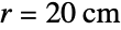 ,长
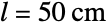 的转动的钢制圆柱体上. 圆柱体要转多快才能储存
 的能量,假定钢的密度为
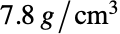 :
cyl = Cylinder[{{0, 0, 0}, {50, 0, 0}}, 20];Graphics3D[{{Opacity[0.5], cyl}, {Red, Arrow[Tube[{{0, 0, 0}, {70, 0, 0}}]]}}, ImageSize -> Small]ρ = Quantity[7.8, "Grams" / "Centimeters" ^ 3];
ℐ = ρ Quantity[MomentOfInertia[cyl, {0, 0, 0}, {1, 0, 0}], "Centimeters" ^ 5]
Solve[(ℐ ω^2/2) == Quantity[1, "KilowattHours"] && ω > 0, ω]UnitConvert[Quantity[ω , "Radians"] /. First[%], "rpm"]刚体的动能由  给出,其中
 为一个角速度向量,
 为转动惯量矩阵. 求一个边长为 2, 4 和 6 的长方体围绕不同的轴的转动能量. 对所有情况,旋转体的质量都是相同的,但对于不同转动轴,质量的分布却是不同的,它是用转动惯量来表示的:
ℐ = MomentOfInertia[Cuboid[{-1, -2, -3}, {1, 2, 3}], {0, 0, 0}]
{1, 0, 0}.ℐ.{1, 0, 0}Graphics3D[{{Opacity[0.5], Cuboid[{-1, -2, -3}, {1, 2, 3}]}, {Red, Arrow[Tube[{{0, 0, 0}, {3, 0, 0}}]]}}]
{0, 1, 0}.ℐ.{0, 1, 0}Graphics3D[{{Opacity[0.5], Cuboid[{-1, -2, -3}, {1, 2, 3}]}, {Green, Arrow[Tube@{{0, 0, 0}, {0, -4, 0}}]}}]
{0, 0, 1}.ℐ.{0, 0, 1}Graphics3D[{{Opacity[0.5], Cuboid[{-1, -2, -3}, {1, 2, 3}]}, {Blue, Arrow[Tube@{{0, 0, 0}, {0, 0, 5}}]}}]一个转动刚体所受力矩  和角加速度
 的关系是
 ,其中
 为转动惯量. 计算一个边长为一米的铅制正方体在角加速度为
 时所需要的力矩:
cube = Cuboid[{-1 / 2, -1 / 2, -1 / 2}, {1 / 2, 1 / 2, 1 / 2}];
Graphics3D[{{Opacity[0.5], cube}, {Red, Arrow[Tube@{{0, 0, -1}, {0, 0, 1}}]}}]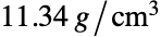
ρ = Quantity[11.34, "Grams" / "Centimeters" ^ 3];
ℐ = ρ Quantity[MomentOfInertia[cube, {0, 0, 0}, {0, 0, 1}], "Meters" ^ 5]α = Quantity[1, 1 / "Seconds" ^ 2];
τ = ℐ αUnitConvert[%, "Newtons" * "Meters"]平行轴定理给出了围绕某一个轴的转动惯量  和围绕一个通过质心且与其平行的轴的转动惯量
 之间的一个关系
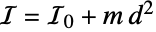 ,其中
 为总质量,
 为两轴之间的距离:
body = Cylinder[{{1, 2, 3}, {4, 5, 6}}, 7];
c = RegionCentroid[body];
p = {2, 2, 2};
v = {2, 1, 0};axis = InfiniteLine[p, v];
axis0 = InfiniteLine[c, v];
Graphics3D[{{Opacity[0.5], body}, {Green, axis}, {Blue, axis0}, {Red, Point[c]}}]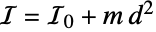
MomentOfInertia[body, p, v] == MomentOfInertia[body, c, v] + RegionMeasure[body] RegionDistance[axis, c] ^ 2属性和关系 (11)
如果省略了转动点,则以 RegionCentroid 为默认值:
body = Cuboid[];MomentOfInertia[body] == MomentOfInertia[body, RegionCentroid[body]]对于一个给定的点  ,将物体平移
 后再计算其相对原点的转动惯量将得到相同的结果:
body = Cylinder[];
pt = {1, 2, 3};MomentOfInertia[body, pt] == MomentOfInertia[TransformedRegion[body, TranslationTransform[-pt]], {0, 0, 0}]body = Pyramid[{{0, 0, 0}, {2, 0, 0}, {2, 2, 0}, {0, 2, 0}, {1, 1, 2}}];
pt = {1, 1, 1}; v = {1, 2, 3};Integrate[RegionDistance[InfiniteLine[pt, v], {x, y, z}] ^ 2, {x, y, z}∈body] == MomentOfInertia[body, pt, v]body = Tetrahedron[{{1, 0, 0}, {1, 0, 1}, {1, 1, 1}, {0, 0, 1}}];Integrate[{{y ^ 2 + z ^ 2, -x y, -x z}, {-y x, x ^ 2 + z ^ 2, -y z}, {-z x, -z y, x ^ 2 + y ^ 2}}, {x, y, z}∈body] == MomentOfInertia[body, {0, 0, 0}]用 Integrate 来计算一个具有变质量密度 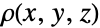 的物体的转动惯量:
body = Ball[{0, 0, 0}, r];ρ = Exp[-x^2]Exp[-y^2]Exp[-z^2];Integrate[{{y ^ 2 + z ^ 2, -x y, -x z}, {-y x, x ^ 2 + z ^ 2, -y z}, {-z x, -z y, x ^ 2 + y ^ 2}}ρ, {x, y, z}∈body, Assumptions -> r > 0]MomentOfInertia[Parallelepiped[{0, 0, 0}, {{1, 0, 0}, {1, 1, 0}, {0, 1, 1}}]]SymmetricMatrixQ[%]MomentOfInertia[Tetrahedron[{{1, 0, 0}, {1, 0, 1}, {1, 1, 1}, {0, 0, 1}}]]PositiveSemidefiniteMatrixQ[%]二维时的转动惯量矩阵可以用 RegionMoment 来计算:
reg = Ellipsoid[{1, 2}, {{1, 2}, {-3, 2}}];
reg0 = TransformedRegion[reg, TranslationTransform[-RegionCentroid[reg]]];
m[ind_] := RegionMoment[reg0, ind]{{m[{0, 2}], -m[{1, 1}]}, {-m[{1, 1}], m[{2, 0}]}}MomentOfInertia[reg] == %三维时的转动惯量矩阵可以用 RegionMoment 来计算:
reg = Parallelepiped[{1, 2, 3}, {{1, 1, 0}, {1, 0, 1}, {0, 1, 1}}];
reg0 = TransformedRegion[reg, TranslationTransform[-RegionCentroid[reg]]];
m[ind_] := RegionMoment[reg0, ind]{{m[{0, 2, 0}] + m[{0, 0, 2}], -m[{1, 1, 0}], -m[{1, 0, 1}]}, {-m[{1, 1, 0}], m[{2, 0, 0}] + m[{0, 0, 2}], -m[{0, 1, 1}]}, {-m[{1, 0, 1}], -m[{0, 1, 1}], m[{2, 0, 0}] + m[{0, 2, 0}]}}MomentOfInertia[reg] == %一个点 Point 的转动惯量为这个点到轴的距离的平方:
point = {1, 2, 3};
pt = {0, 0, 0};
v = {1, 1, 1};
axis = InfiniteLine[pt, v];MomentOfInertia[Point@point, pt, v] == RegionDistance[axis, point] ^ 2pts = Tuples[Range[5], 3];MomentOfInertia[Point@pts, pt, v] == Total[RegionDistance[axis, pts] ^ 2]bodies = {Cuboid[], Ball[{2, 2, 2}]};
pt = {0, 0, 0};
v = {1, 1, 1};MomentOfInertia[RegionUnion@@bodies, pt, v] == Total[MomentOfInertia[#, pt, v]& /@ bodies]Graphics3D[{{Opacity[0.7], bodies}, {Red, InfiniteLine[pt, v]}}]文本
Wolfram Research (2016),MomentOfInertia,Wolfram 语言函数,https://reference.wolfram.com/language/ref/MomentOfInertia.html.
CMS
Wolfram 语言. 2016. "MomentOfInertia." Wolfram 语言与系统参考资料中心. Wolfram Research. https://reference.wolfram.com/language/ref/MomentOfInertia.html.
APA
Wolfram 语言. (2016). MomentOfInertia. Wolfram 语言与系统参考资料中心. 追溯自 https://reference.wolfram.com/language/ref/MomentOfInertia.html 年