Series, Limits, and Residues
| Sum[f,{i,imin,imax}] | the sum |
| Sum[f,{i,imin,imax,di}] | the sum with i increasing in steps of di |
| Sum[f,{i,imin,imax},{j,jmin,jmax}] | the nested sum |
| Product[f,{i,imin,imax}] | the product |
The Wolfram Language also has a notation for multiple sums and products. Sum[f,{i,imin,imax},{j,jmin,jmax}] represents a sum over i and j, which would be written in standard mathematical notation as  . Notice that in Wolfram Language notation, as in standard mathematical notation, the range of the outermost variable is given first.
This is the multiple sum  . Notice that the outermost sum over i is given first, just as in the mathematical notation:
The way the ranges of variables are specified in Sum and Product is an example of the rather general iterator notation that the Wolfram Language uses. You will see this notation again when we discuss generating tables and lists using Table ("Making Tables of Values"), and when we describe Do loops ("Repetitive Operations").
| {imax} | iterate imax times, without incrementing any variables |
| {i,imax} | i goes from 1 to imax in steps of 1 |
| {i,imin,imax} | i goes from imin to imax in steps of 1 |
| {i,imin,imax,di} | i goes from imin to imax in steps of di |
| {i,imin,imax},{j,jmin,jmax},… | i goes from imin to imax, and for each such value, j goes from jmin to jmax, etc. |
The mathematical operations we have discussed so far are exact. Given precise input, their results are exact formulas.
In many situations, however, you do not need an exact result. It may be quite sufficient, for example, to find an approximate formula that is valid, say, when the quantity x is small.
If you give it a function that it does not know, Series writes out the power series in terms of derivatives:
Power series are approximate formulas that play much the same role with respect to algebraic expressions as approximate numbers play with respect to numerical expressions. The Wolfram Language allows you to perform operations on power series, in all cases maintaining the appropriate order or "degree of precision" for the resulting power series.
When you do operations on a power series, the result is computed only to the appropriate order in x:
Applying Expand gives a result with 11 terms:
| Series[expr,{x,x0,n}] | find the power series expansion of expr about the point x=x0 to at most n th order |
| Normal[series] | truncate a power series to give an ordinary expression |
| Series[expr,{x,x0,n}] | find the power series expansion of expr about the point x=x0 to order at most (x-x0)n |
| Series[expr,{x,x0,nx},{y,y0,ny}] | |
find series expansions with respect to y, then x | |
If the Wolfram Language does not know the series expansion of a particular function, it writes the result symbolically in terms of derivatives:
In mathematical terms, Series can be viewed as a way of constructing Taylor series for functions.
The standard formula for the Taylor series expansion about the point  of a function
  with
with  th derivative
  is
is 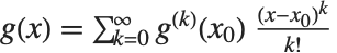 . Whenever this formula applies, it gives the same results as Series. (For common functions, Series nevertheless internally uses somewhat more efficient algorithms.)
Series can also generate some power series that involve fractional and negative powers, not directly covered by the standard Taylor series formula.
Series can also handle series that involve logarithmic terms:
There are, of course, mathematical functions for which no standard power series exist. The Wolfram Language recognizes many such cases.
Especially when negative powers occur, there is some subtlety in exactly how many terms of a particular power series the function Series will generate.
One way to understand what happens is to think of the analogy between power series taken to a certain order, and real numbers taken to a certain precision. Power series are "approximate formulas" in much the same sense as finite‐precision real numbers are approximate numbers.
The procedure that Series follows in constructing a power series is largely analogous to the procedure that N follows in constructing a real‐number approximation. Both functions effectively start by replacing the smallest pieces of your expression by finite‐order, or finite‐precision, approximations, and then evaluating the resulting expression. If there are, for example, cancellations, this procedure may give a final result whose order or precision is less than the order or precision that you originally asked for. Like N, however, Series has some ability to retry its computations so as to get results to the order you ask for. In cases where it does not succeed, you can usually still get results to a particular order by asking for a higher order than you need.
Series compensates for cancellations in this computation, and succeeds in giving you a result to order  :
:
When you make a power series expansion in a variable x, the Wolfram Language assumes that all objects that do not explicitly contain x are in fact independent of x. Series thus does partial derivatives (effectively using D) to build up Taylor series.
You can use Series to generate power series in a sequence of different variables. Series works like Integrate, Sum, and so on, and expands first with respect to the last variable you specify.
Series performs a series expansion successively with respect to each variable. The result in this case is a series in x, whose coefficients are series in y:
Power series are represented in the Wolfram System as SeriesData objects.
The power series is printed out as a sum of terms, ending with O[x] raised to a power:
Internally, however, the series is stored as a SeriesData object:
By using SeriesData objects, rather than ordinary expressions, to represent power series, the Wolfram System can keep track of the order and expansion point, and do operations on the power series appropriately. You should not normally need to know the internal structure of SeriesData objects.
You can recognize a power series that is printed out in standard output form by the presence of an O[x] term. This term mimics the standard mathematical notation  , and represents omitted terms of order
  . For various reasons of consistency, the Wolfram System uses the notation O[x]^n for omitted terms of order
  , corresponding to the mathematical notation
  , rather than the slightly more familiar, though equivalent, form
  .
.
Any time that an object like O[x] appears in a sum of terms, the Wolfram System will in fact convert the whole sum into a power series.
The presence of O[x] makes the Wolfram System convert the whole sum to a power series:
The logarithmic factors appear explicitly inside the SeriesData coefficient list:
The Wolfram Language allows you to perform many operations on power series. In all cases, the Wolfram Language gives results only to as many terms as can be justified from the accuracy of your input.
The Wolfram Language keeps track of the orders of power series in much the same way as it keeps track of the precision of approximate real numbers. Just as with numerical calculations, there are operations on power series which can increase, or decrease, the precision (or order) of your results.
When you perform an operation that involves both a normal expression and a power series, the Wolfram Language "absorbs" the normal expression into the power series whenever possible.
If you add Sin[x], the Wolfram Language generates the appropriate power series for Sin[x], and combines it with the power series you have:
The Wolfram Language also absorbs expressions that multiply power series. The symbol a is assumed to be independent of x:
The Wolfram Language knows how to apply a wide variety of functions to power series. However, if you apply an arbitrary function to a power series, it is impossible for the Wolfram Language to give you anything but a symbolic result.
The Wolfram Language does not know how to apply the function f to a power series, so it just leaves the symbolic result:
When you manipulate power series, it is sometimes convenient to think of the series as representing functions, which you can, for example, compose or invert.
| ComposeSeries[series1,series2,…] | compose power series |
| InverseSeries[series,x] | invert a power series |
If you have a power series for a function  , then it is often possible to get a power series approximation to the solution for
  in the equation
  . This power series effectively gives the inverse function
  such that
  . The operation of finding the power series for an inverse function is sometimes known as reversion of power series.
| Normal[expr] | convert a power series to a normal expression |
Power series in the Wolfram Language are represented in a special internal form, which keeps track of such attributes as their expansion order.
For some purposes, you may want to convert power series to normal expressions. From a mathematical point of view, this corresponds to truncating the power series, and assuming that all higher‐order terms are zero.
Normal truncates the power series, giving a normal expression:
| SeriesCoefficient[series,n] | give the coefficient of the n th order term in a power series |
| LogicalExpand[series1==series2] | give the equations obtained by equating corresponding coefficients in the power series |
| Solve[series1==series2,{a1,a2,…}] | solve for coefficients in power series |
This solves the equations for the coefficients a[i]. You can also feed equations involving power series directly to Solve:
Some equations involving power series can also be solved using the InverseSeries function discussed in "Composition and Inversion of Power Series".
| Sum[expr,{n,nmin,nmax}] | find the sum of expr as n goes from nmin to nmax |
There are many analogies between sums and integrals. And just as it is possible to have indefinite integrals, so indefinite sums can be set up by using symbolic variables as upper limits.
The Wolfram System can do essentially all sums that are found in books of tables. Just as with indefinite integrals, indefinite sums of expressions involving simple functions tend to give answers that involve more complicated functions. Definite sums, like definite integrals, often, however, come out in terms of simpler functions.
If you represent the n th term in a sequence as a[n], you can use a recurrence equation to specify how it is related to other terms in the sequence.
| RSolve[eqn,a[n],n] | solve a recurrence equation |
RSolve can be thought of as a discrete analog of DSolve. Many of the same functions generated in solving differential equations also appear in finding symbolic solutions to recurrence equations.
RSolve does not require you to specify explicit values for terms such as a[1]. Like DSolve, it automatically introduces undetermined constants C[i] to give a general solution.
RSolve can solve equations that do not depend only linearly on a[n]. For nonlinear equations, however, there are sometimes several distinct solutions that must be given. Just as for differential equations, it is a difficult matter to find symbolic solutions to recurrence equations, and standard mathematical functions only cover a limited set of cases.
RSolve can solve not only ordinary difference equations in which the arguments of  differ by integers, but also
  ‐difference equations in which the arguments of
  are related by multiplicative factors.
| RSolve[{eqn1,eqn2,…},{a1[n],a2[n],…},n] | |
solve a coupled system of recurrence equations | |
| RSolve[eqns,a[n1,n2,…],{n1,n2,…}] | |
solve partial recurrence equations | |
Just as one can set up partial differential equations that involve functions of several variables, so one can also set up partial recurrence equations that involve multidimensional sequences. Just as in the differential equations case, general solutions to partial recurrence equations can involve undetermined functions.
In doing many kinds of calculations, you need to evaluate expressions when variables take on particular values. In many cases, you can do this simply by applying transformation rules for the variables using the /. operator.
Consider, for example, finding the value of the expression  when
when  . If you simply replace
  by
by  in this expression, you get the indeterminate result
  . To find the correct value of
  when
when  , you need to take the limit.
| Limit[expr,x->x0] | find the limit of expr when x approaches x0 |
Not all functions have definite limits at particular points. For example, the function  oscillates infinitely often near
  , so it has no definite limit there. Nevertheless, at least so long as
  remains real, the values of the function near
  always lie between
  and
and  . Limit represents values with bounded variation using Interval objects. In general, Interval[{xmin,xmax}] represents an uncertain value which lies somewhere in the interval
  to
to  .
.
Limit returns an Interval object, representing the range of possible values of  near its essential singularity at
  :
:
The Wolfram Language can do arithmetic with Interval objects:
The Wolfram Language represents this limit symbolically in terms of an Interval object:
Some functions may have different limits at particular points, depending on the direction from which you approach those points. You can use the Direction option for Limit to specify the direction you want.
| Limit[expr,x->x0,Direction->1] | find the limit as x approaches x0 from below |
| Limit[expr,x->x0,Direction->-1] | find the limit as x approaches x0 from above |
The function  has a different limiting value at
  , depending on whether you approach from above or below:
Limit makes no assumptions about functions like f[x] about which it does not have definite knowledge. As a result, Limit remains unevaluated in most cases involving symbolic functions.
Limit[expr,x->x0] tells you what the value of expr is when x tends to x0. When this value is infinite, it is often useful instead to know the residue of expr when x equals x0. The residue is given by the coefficient of  in the power series expansion of expr about the point x0.
| Residue[expr,{x,x0}] | the residue of expr when x equals x0 |
The Padé approximation is a rational function that can be thought of as a generalization of a Taylor polynomial. A rational function is the ratio of polynomials. Because these functions only use the elementary arithmetic operations, they are very easy to evaluate numerically. The polynomial in the denominator allows you to approximate functions that have rational singularities.
| PadeApproximant[f,{x,x0,{n,m}}] | give the Padé approximation to |
| PadeApproximant[f,{x,x0,n}] | give the diagonal Padé approximation to |
More precisely, a Padé approximation of order  to an analytic function
  at a regular point or pole
  is the rational function
  where
where  is a polynomial of degree
  ,
,  is a polynomial of degree
  , and the formal power series of
  about the point
  begins with the term
  . If
. If  is equal to
  , the approximation is called a diagonal Padé approximation of order
  .
.
The initial terms of this series vanish. This is the property that characterizes the Padé approximation:
This plots the difference between the approximation and the true function. Notice that the approximation is very good near the center of expansion, but the error increases rapidly as you move away:
In the Wolfram Language PadeApproximant is generalized to allow expansion about branch points.