Hierarchical Model—Tank System
Installation and Setup | Introduction | Multidomain | Components | Custom Components | Hello World | External Functions | Hierarchical Models | Systems
This example illustrates how you can build a hierarchical model using System Modeler, as well as how to make new libraries. A flat tank model is first developed, followed by a similar component-based tank model. We then see the flexibility that this gives us to test new scenarios.
MODELS USED IN THIS TUTORIAL |
| FlatTank TankPI TankPID TankSystem |
Flat Tank
The system we will begin with is a one-tank system with a controller, as illustrated in the picture below.
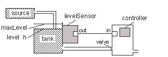
Graphical representation of a tank system.
To implement the model, we need to set up the system equations. The water level h in the tank is a function of the flow in and out of the tank and the tank area:
In this example, we choose an input flow that is constant during the first 150 seconds, after which it triples. In the following expression for qin(t), q0 is a parameter:
By controlling the output flow, we will try to keep the tank level at a desired reference value ref. In order to do this, we implement a PI controller where e is the control error, K is the controller gain, and T is the time constant of the controller:
The controller demands a flow u into the tank, and since it controls the flow via the output valve, this is a demanded value for -qout. However, the actual output flow qout is limited by a minimum value minFlow and a maximum value maxFlow, and we observe that qout cannot exceed qin when the tank is empty. With this information, we can implement the flat Modelica code.
model FlatTank "Flat model of a tank"
  parameter Real q0(unit = "m3/s") = 0.15 "Scaling of input flow";
  parameter Real A(unit = "m2") = 1 "Tank bottom area";
  parameter Real K(unit = "V/m") = 0.1 "PI controller gain";
  parameter Real T(unit = "s") = 10 "PI controller integrator time constant";
  parameter Real minFlow(unit = "m3/s") = 0 "Minimum flow through output valve";
  parameter Real maxFlow(unit = "m3/s") = 0.5 "Maximum flow through output valve";
  parameter Real ref(unit = "m") = 0.25 "Reference level for control";
  Real h(start = 0, unit = "m") "Tank level";
  Real qIn(unit = "m3/s") "Flow through input valve";
  Real qOut(unit = "m3/s") "Flow through output valve";
  Real qOutMax(unit = "m3/s") "Maximum output flow considering that the tank level cannot be negative";
  Real u(unit = "m3/s") "Output flow demanded by controller";
  Real e(unit = "m") "Deviation from reference level";
  Real x(unit = "m") "State variable for controller";
equation
  assert(minFlow >= 0, "minFlow - minimum flow through output valve must be >= 0");
  der(h) = (qIn - qOut) / A;
  qIn = if time > 150 then 3 * q0 else q0;
  qOutMax = if h > 0 then maxFlow else min(qIn, maxFlow);
  qOut = if (-u) < minFlow then minFlow elseif (-u) > qOutMax then qOutMax else -u;
  e = ref - h;
  der(x) = e / T;
  u = K * (e + x);
end FlatTank;
By simulating the model for 350 seconds, we can see that the tank level starts to increase, reaching and then surpassing the desired reference level. Once the desired level is surpassed, the outflow is opened, and somewhere around 100 seconds the level stabilizes. However, at 150 seconds the input flow is suddenly increased, and this time it takes longer to stabilize the tank level due to saturation of the control signal. This is illustrated in the figure below.
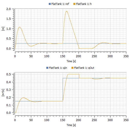
Plotting the tank level and the flows in and out of the flat tank with default parameter values.
Component-Based Tank
Implementing a component-based tank will require a bit more work to begin with, but as soon as we start experimenting with the tank and testing different scenarios we will regain the invested time.
When using the object-oriented component-based approach to modeling, we first try to understand the system structure and decomposition in a hierarchical top-down manner. Once the system components and interactions between these components have been roughly identified, we can apply the first traditional modeling phases of identifying variables and equations to each of these model components.
By studying the figure in the beginning of this chapter, we see that the tank system has a natural component structure.
We can identify five components in the figure: the tank itself, the liquid source, the level sensor, the valve, and the controller. However, since we will choose very simple representations of the level sensor and the valve, i.e. just a simple scalar variable for each, we let these variables be simple variables of type Real in the tank model instead of creating two new classes, each containing a single variable.
The next step is to determine the interactions and communication paths between the components. It is fairly obvious that liquid flows from the source tank via a pipe. Liquid also leaves the tank via an outlet controlled by the valve. The controller needs measurements of the liquid level from the sensor. Thus, a communication path from the sensor of the tank and the controller needs to be established.
In order to connect communication paths, connector instances must be created for those components that are connected, and connector classes must be declared when needed. In fact, the system model should be designed such that the only communication between a component and the rest of the system is via connectors.
Finally, we should think about reuse and generalizations of certain components. For example, do we expect that several variants of a component will be needed? In the case of the tank system, we expect to plug in several variants of the controller, starting with a PI controller. Thus, it is useful for us to create a base class for tank system controllers.
The structure of the tank system model developed using the object-oriented component-based approach is clearly visible in the figure below.
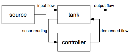
Graphical representation of an object-oriented component-based tank system.
We can identify three different types of classes that will be used in the model: interfaces, functions, and components. Therefore, we develop a package containing three subpackages. To create a package, right-click the User Classes root in the Class Browser and select New Class, as shown in the screenshot below. You can also right-click the package in which you want to add your package and select New Class....
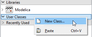
In the dialog box that opens, set the class specialization to Package and give the package the name Hierarchical. Click the OK button to create the new package. The package will appear in the User Classes tree of the Class Browser. By right-clicking the name of the new package, we can create and add models and packages to it.
Interfaces
We are now ready to create the interfaces, called connectors. Begin by creating a new package Interfaces within the Hierarchical package. Unless already expanded, expand the Hierarchical package in the Class Browser to view its contents. Create connector classes within the Interfaces package using the New Class dialog. Besides the name of the class, specify Connector as the class specialization, type Real in the Extends field, and tick the Short class definition checkbox to get the basic parts of the definition right.
Create connector classes for the tank level reading. Begin with the input connector and call it ReadSignalInput in the New Class dialog.
Modify the definition by typing input before Real to specify the direction of the connector, specify the unit to be meters, and add a suitable documentation string (see the HelloWorld example to see how to edit models textually and make model icons).
Create a matching output connector by duplicating the input connector and making minor changes.
We also need connector classes for the signal to the actuator for demanded flow. Begin with the input connector.
connector ActSignalInput = input Real(unit = "m3/s") "Input of signal to actuator for setting valve position";
Again, create a matching output connector.
connector ActSignalOutput = output Real(unit = "m3/s") "Output of signal to actuator for setting valve position";
Finally, we also need connector classes for the liquid flow at inlets and outlets. The physical nature of the system, with liquid flowing only in one direction from one compartment to the next, allows us to use the same type of input and output connectors as for the tank level reading and the actuator signal. If the causality of the liquid flow would not have been that obvious, it might have been necessary to use an acausal connector containing both flow and pressure variables.
Although the actuator signal and liquid flow connectors use the same unit (so that their definitions will be identical up to naming), we still make a distinction between the two types of connectors as they serve different purposes. The former are for communicating a control signal, and the latter represent an actual flow of liquid. Begin with the input connector.
Again, create a matching output connector.
Tank Components
The next step is to create the three components of the system. Begin by creating a Components package within the Hierarchical package. In the Components package, create a tank model named Tank. The tank model has four interfaces (connectors in Modelica): qIn for input flow, qOut for output flow, y for providing tank level measurements, and u for demanding a flow through the valve at the outlet of the tank. The central equation regulating the behavior of the tank is the mass balance equation, which in the current simple form assumes constant pressure. The output flow is related to the demanded flow via a sign change and physical limitations that we handle using the LimitValue function.
model Tank "Model of a simple tank holding liquid"
  parameter Real A(unit = "m2") = 1 "Bottom area";
  parameter Real minFlow(unit = "m3/s") = 0 "Minimum flow through output valve";
  parameter Real maxFlow(unit = "m3/s") = 0.5 "Maximum flow through output valve";
  Interfaces.ActSignalInput u "Actuator controlling output flow, connector";
  Interfaces.LiquidFlowInput qIn "Flow through input valve, connector";
  Interfaces.ReadSignalOutput y "Sensor reading tank level, connector";
  Interfaces.LiquidFlowOutput qOut "Flow through output valve, connector";
  Real h(start = 0.0, unit = "m") "Liquid level";
  Real qOutMax(unit = "m3/s") "Maximum output flow considering that the tank level cannot be negative";
equation
  assert(minFlow >= 0, "minFlow - minimum flow through output valve must be >= 0");
  der(h) = (qIn - qOut) / A;
  qOutMax = if h > 0 then maxFlow else min(qIn, maxFlow);
  qOut = Functions.LimitValue(minFlow, qOutMax, -u);
  y = h;
end Tank;
The model uses the already defined connectors as well as the LimitValue function, which has not been defined yet. This is defined by creating the following function within a new package, named Functions. As it is a function, we set its class specialization to Function when creating it. To allow the numeric solver to determine exactly where the limited value is crossing any of the boundaries, we use the Inline and GenerateEvents annotations.
function LimitValue "Limiting function"
  input Real pMin;
  input Real pMax;
  input Real p;
  output Real pLim;
algorithm
  pLim := if p < pMin then pMin elseif p > pMax then pMax else p;
  annotation(Inline = true, GenerateEvents = true);
end LimitValue;
The liquid entering the tank must originate somewhere. Therefore, we have a liquid source component that starts with a constant output flow that then increases sharply at t=150 by a factor of three. This creates an interesting control problem that the tank controller must handle. The following model is created in the Components package.
model LiquidSource "Source of liquid with varying output"
  parameter Real q0(unit = "m3/s") = 0.15 "Scaling of input flow";
  Interfaces.LiquidFlowOutput qOut "Output flow, connector";
equation
 qOut = if time > 150 then 3 * q0 else q0;
end LiquidSource;
Controllers
Finally, the controllers need to be specified. We will initially choose a PI controller, but may later replace it with other kinds of controllers. The behavior of the PI (proportional and integrating) controller in the flat model was defined by the following two equations:
This time, the two equations are placed in the controller class PIController, which extends the BaseController class defined later.
model PIController "Elementary PI controller"
  extends BaseController;
  parameter Real K(unit = "m2/s") = 0.1 "Gain";
  parameter Real T(unit = "s") = 10 "Integrator time constant";
  Real x(unit = "m") "Integrator state";
equation
  der(x) = e / T;
  u = K * (e + x);
end PIController;
Both the PI and PID controllers to be defined later inherit the partial controller class BaseController, containing common parameters, state variables, and two connectors: one to read the sensor and one to control the valve actuator.
partial model BaseController "Base class for tank level controllers"
  parameter Real ref(unit = "m") "Reference level";
  Interfaces.ActSignalOutput u "Control to actuator, connector";
  Interfaces.ReadSignalInput y "Input sensor level, connector";
  Real e(unit = "m") "Deviation from reference level";
equation
  e = ref - y;
end BaseController;
Small Tank System
When this is finished, we can compose our tank system model with drag-and-drop.
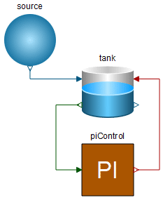
The Diagram View of the IntroductoryExamples.Hierarachical.TankPI model.
Simulating for 350 seconds yields the same result as the flat tank system.
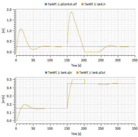
Plotting the tank level and the flows in and out of the PI-controlled tank with default parameter values.
Tank with PID Controller
We now define a TankPID system, which is the same as the TankPI system except that the PI controller has been replaced by a PID controller. Here we see a clear advantage of the object-oriented component-based approach over the traditional model-based approach, since system components can easily be replaced and changed in a plug-and-play manner.
A PID (proportional, integrating, derivating) controller model can be derived in a similar way as the PI controller. The basic PID control law used here is:
It is implemented using the following equations:
Using these equations and the BaseController class, we create the PID controller.
model PIDController "Elementary PID controller"
  extends BaseController;
  parameter Real K(unit = "m2/s") = 0.1 "Gain";
  parameter Real T(unit = "s") = 10 "Integrator time constant";
  parameter Real Td(unit = "s") = 5 "Derivative gain";
  Real x(unit = "m") "Integrator state";
equation
  der(x) = e / T;
  u = K * (e + x + Td * der(e));
end PIDController;
We can now compose a PID-controlled tank system using drag-and-drop.
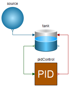
Diagram View of the IntroductoryExamples.Hierarchical.TankPID model.
We simulate for 350 seconds again and compare with the previous result.
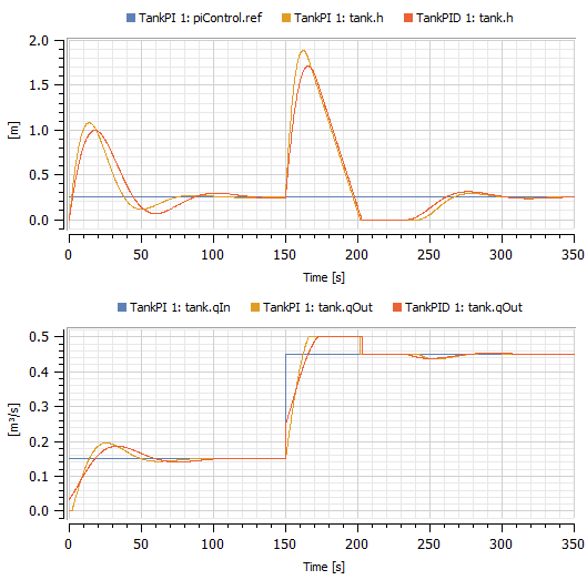
Comparison of tank levels between the TankPI model and the TankPID model.
Three Tank System
Finally, thanks to the object-oriented component-based approach, we can compose a larger system with ease.
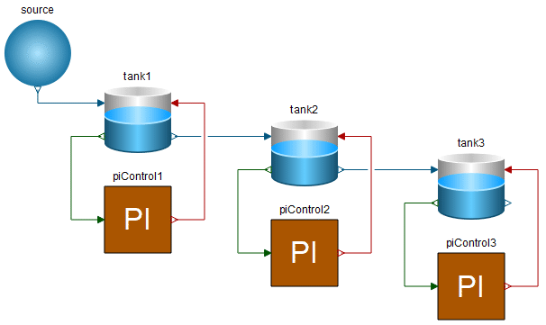
Diagram View of the IntroductoryExamples.Hierarchical.TankSystem model.
Simulating this system, we can study how the level of each tank is controlled.
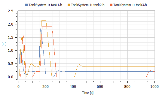
Evolution of the tank levels from the TankSystem model.
Note that the second tank has a reference level of 0.4 meters, while the other tanks have a reference level of 0.2 meters. Problems with integrator windup in the PI controllers lead to a poor response to the change in input flow after 150 seconds, requiring 1000 seconds of total simulation time to capture the essential parts of the behavior.
Next Chapter
Installation and Setup | Introduction | Multidomain | Components | Custom Components | Hello World | External Functions | Hierarchical Models | Systems
