1.2.3 An Example Application

This example describes the standard way how to use Analog Insydes. It can easily be adapted to different analysis tasks and applications. The usage of many different commands, from netlist import to linear simplification techniques, is explained and cross references are given where to find more information. Reading this section should give you a first overview of the capabilities of Analog Insydes.

Analysis Task

Following, we want to analyze the operational amplifier. The task is to find an interpretable symbolic formula for the corner frequency of the small-signal voltage transfer function. This is useful to identify those circuit elements and parasitics, which have a dominant influence on it. In addition, the symbolic transfer function can be utilized for further investigation, such as the extraction of its poles and zeros, to find methods for the compensation of certain effects.

Importing Schematics

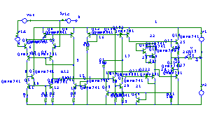
To import the schematics picture of the operational amplifier, we use the Analog Insydes command DXFGraphics. This command translates two-dimensional DXF data into Mathematica graphics objects which can be displayed in a Mathematica notebook. Most schematics entries of commercial circuit simulators support the export of schematics in DXF format. DXFGraphics allows for importing your schematics into Mathematica for documentation purposes.

Before using DXFGraphics, of course we have to load the Analog Insydes master package as described in Section 1.2.2.

In[1]:= <<AnalogInsydes`

In[2]:= DXFGraphics["AnalogInsydes/DemoFiles/OP-741.dxf"]

Out[2]=

DXFGraphics provides many options for altering the appearance of imported DXF files. They are described in Section 3.13.2.

Importing Netlist Data

For the application of symbolic analysis, especially symbolic approximation, the next step is to generate a netlist including the numerical reference information. The netlist of the operational amplifier consists of 45 elements. Writing the complete circuit in the Analog Insydes netlist language (which is described in Chapter 2.2 and Chapter 2.3) by hand would be a tedious and error-prone task. Therefore, Analog Insydes provides the command ReadNetlist, which automatically translates an external netlist description into the Analog Insydes netlist format. You can import netlists written for or generated by PSpice, Eldo, and Saber.

The first argument to ReadNetlist is the simulator input file. Since this file (*.cir in our case) only contains the numerical values of the elements, the operating-point information and the values for the small-signal parameters of the transistors have to be extracted from the simulator output file (*.out in our case). This is performed automatically by ReadNetlist, too. All we have to do is specifying the corresponding simulator output file as second argument.

In[3]:= op741 = ReadNetlist[
"AnalogInsydes/DemoFiles/OP-741.cir",
"AnalogInsydes/DemoFiles/OP-741.out",
Simulator -> "PSpice", KeepPrefix -> False]

Out[3]=

As the syntax of external netlist files varies for each simulator, you have to specify from which external format you are reading by means of the Simulator option of ReadNetlist.

The return value of ReadNetlist is a Circuit object which contains symbolic values for each netlist element as well as the corresponding numerical reference information. By default, the Circuit object is displayed as a single line in your output cell. To view the complete netlist apply the command DisplayForm to the Circuit object:

DisplayForm[op741]

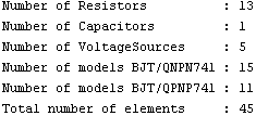
Additionally, you can use the command Statistics to get an impression of the circuit complexity. This command prints the number of different element types occuring in the circuit.

In[4]:= Statistics[op741]

Setting Up Circuit Equations

Once the netlist is imported, the next step is to set up the symbolic circuit equations. In Analog Insydes this can be done automatically using the command CircuitEquations. The Analog Insydes netlist read by ReadNetlist contains generic model references for each transistor and does not specifiy a concrete model implementation. Thus, we have to instruct Analog Insydes which model to use during equation setup by means of the option ModelLibrary. Analog Insydes comes with a predefined SPICE-compatible, symbolic model library in three different complexity levels called "FullModels`", "SimplifiedModels`", and "BasicModels`" (the implemented models are explained in detail in Chapter 4.3. For special tasks the model library can be extended by the user; this topic is discussed in Chapter 2.3). In the following, we choose a complexity-reduced BJT model from the Analog Insydes model library by setting the option ModelLibrary -> "BasicModels`". Note that a quote mark ("`") is following the word BasicModels.

In[5]:= mnaAC741 = CircuitEquations[op741,
ElementValues -> Symbolic,
ModelLibrary -> "BasicModels`"]

Out[5]=

The additional option ElementValues -> Symbolic tells Analog Insydes to set up equations using the symbolic element values instead of the numerical ones. By default, CircuitEquations sets up small-signal equations in matrix formulation, but DC or transient equations can be set up, too. See Section 3.5.1 and Chapter 2.4 for details. CircuitEquations returns a DAEObject which contains the equation system as well as additional data which is used and extracted automatically by other Analog Insydes commands. As for Circuit objects, a DAEObject is printed in short notation only and can be displayed using DisplayForm:

DisplayForm[mnaAC741]

Again, you can use Statistics to get an impression of the equation size.

In[6]:= Statistics[mnaAC741]

Importing Simulation Data

When using netlists from external simulators we always have to verify that the models used during equation setup are compatible to the ones used by the simulator. This is done by comparing the numerical solution calculated by the external simulator with the solution calculated by Analog Insydes. If both solutions do not coincide within a tolerable error range, we have to go back one step and choose different models during equation setup before going on with the symbolic analysis. To simplify this procedure, Analog Insydes provides the command ReadSimulationData for importing numerical data generated by an external simulator. As for ReadNetlist we have to specify from which format we are reading by means of the Simulator option. The list of supported formats is shown in Section 3.10.1.

In[7]:= op741data = ReadSimulationData[
"AnalogInsydes/DemoFiles/OP-741.csd",
Simulator -> "PSpice"]

Out[7]=

ReadSimulationData returns the result according to the Analog Insydes numerical data format which is described in Section 3.7.1. It consists of a list of rules, where the variables (which are returned as strings) are assigned InterpolatingFunction objects.

Graphically Displaying Simulation Data

We can use Mathematica's ReplaceAll operator (or /. in short notation) to extract a single interpolating function from the numerical data and assign it to a new variable.

In[8]:= vout741PSpice = "V(26)" /. First[op741data]

Out[8]=

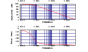
The variable vout741PSpice now contains the numerical data for the output voltage at node 26. Its waveform can be graphically displayed in a Bode diagram using the function BodePlot.

In[9]:= BodePlot[vout741PSpice[f], {f, 0.1, 10^6}]

Out[9]=

Analog Insydes provides several standard graphic functions for visualizing numerical analysis results, see Chapter 2.5 and Chapter 3.9.

Performing Reference Simulation

A numerical reference simulation is performed applying the Analog Insydes function ACAnalysis in the frequency range of interest. The first argument of ACAnalysis is the DAEObject created by CircuitEquations, which contains the system of equations. The second argument denotes the output variable to solve for. We are interested in the node voltage at node  and according to the automatic naming mechanism (which is described in Section 2.4.1) the corresponding variable is called V$26.

In[10]:= reference = ACAnalysis[mnaAC741, V$26, {f, 0.1, 10^6}]

Out[10]=

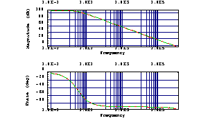
Next, the frequency response calculated with Analog Insydes and the simulation data imported from PSpice are compared graphically, using the capability of the command BodePlot to display several transfer functions within one plot.

In[11]:= BodePlot[reference, {vout741PSpice[f], V$26[f]},
{f, 0.1, 10^6}, ShowLegend -> False]

Out[11]=

The curves match perfectly in the frequency range of interest. Hence, the simplified BJT model is sufficient for being used in the next step of the symbolic analysis flow.

Calculating the Complexity of the Symbolic Transfer Function

Recall that the task is to calculate the symbolic transfer function in order to extract a formula for the corner frequency. Thus, at this point it is useful to estimate the complexity of the symbolic transfer function to find out whether the number of its terms is manageable. This can be done with the help of the function ComplexityEstimate.

In[12]:= ComplexityEstimate[mnaAC741] // N

Out[12]=

ComplexityEstimate returns an integer value. We use Mathematica`s N operator to transform this integer into a real number. The result shows that the number of terms forming the fully expanded symbolic transfer function is greater than and thus too large to be handled. Therefore, we will now apply a routine which removes all those terms whose influence on the behavior of the transfer function is negligible. This drastically reduces the complexity.

Setting Up Circuit Equations for Approximation

To prepare the simplification process we set up the system of circuit equations again. As against the previous call to the function CircuitEquations, where the circuit equations were given in the modified nodal analysis format, they are set up in sparse tableau formulation this time. Sparse tableau is the preferred equation formulation when performing linear approximation tasks. Details about the Formulation option are given in Section 3.5.1.

In[13]:= staAC741 = CircuitEquations[op741,
ElementValues -> Symbolic, Formulation -> SparseTableau,
ModelLibrary -> "BasicModels`"]

Out[13]=

The returned equation system is a DAEObject with equations and variables.

In[14]:= Statistics[staAC741]

Although this sparse tableau system is more than 10 times bigger than the modified nodal system, it usually produces better approximation results.

Performing Matrix Approximation

Now we call the matrix approximation routine on the symbolic circuit equations of the circuit. This routine simplifies the equations based on numerical constraints with respect to a given output variable. The required information is provided in form of several sampling points, specified in combination with a maximum error constraint each. The approximation routine then processes the matrix such that the sought output function is located within the defined error range around the given sampling points. For further information please refer to Section 3.11.3.

To capture the first corner frequency, we place sampling points at and at with a maximum error of each.

In[15]:= samplingpoints = {{s -> 2. Pi I 1., MaxError -> 0.3},
{s -> 2. Pi I 10., MaxError -> 0.3}}

Out[15]=

With the given setup, the approximation routine can be called. The computation is carried out with respect to the output voltage across the load resistor R13, which in this case is equivalent to the sought transfer function. Again, based on the automatic naming scheme (Section 2.4.1), the corresponding variable is called V$R13 (note that sparse tableau equations consist of branch voltages instead of node voltages).

In[16]:= op741approx = ApproximateMatrixEquation[staAC741, V$R13,
samplingpoints]

Out[16]=

In[17]:= Statistics[op741approx]

As another call to the function Statistics shows, the approximation routine could considerably reduce the complexity of the DAEObject (i.e. the number of non-zero entries), although its equation size did not change. With just a small number of terms remaining, a symbolic computation of the transfer function is now possible.

Calculating the Transfer Function

To calculate the transfer function, we now solve the approximated system of equations for the output voltage:

In[18]:= approximation = Solve[op741approx, V$R13]

Out[18]=

Again, we use Mathematica's ReplaceAll operator to extract the calculated solution and assign it to a new variable.

In[19]:= vout741 = V$R13 /. First[approximation] // Simplify

Out[19]=

This expression now represents the approximated symbolic transfer function of the circuit. It contains only those circuit elements and parasitics that were not removed by the matrix approximation routine. Thus, they have been identified as those elements, which have a major influence on the behavior of the transfer function.

Verifying Approximation Results

The quality of the approximation can be determined by performing a numerical comparison between the simplified transfer function and the data imported from the numerical simulator (PSpice in this case). Therefore, we need to extract the design point from the DAEObject first using the command GetDesignPoint. The design point specifies those numerical values for each one of the circuit elements that were given in the netlist.

In[20]:= designpoint = GetDesignPoint[staAC741]

Out[20]=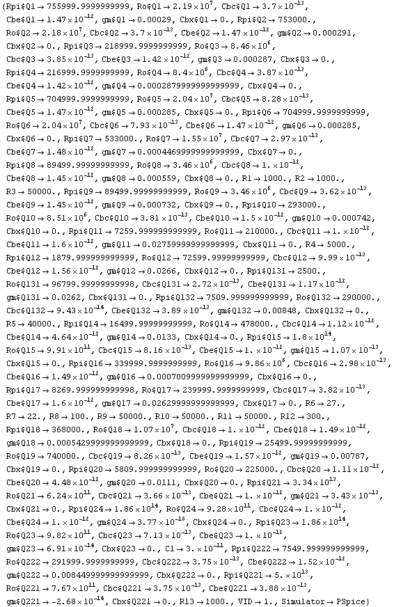

The numerical representation of the approximated transfer function depending on the Laplace variable s is now found by applying the numerical design point data to the symbolic transfer function.

In[21]:= vout741N[s_] = vout741 /. designpoint // Simplify

Out[21]=

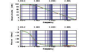
Another Bode plot shows the PSpice simulation data compared with the approximated numeric transfer function in the frequency range from to .

In[22]:= BodePlot[{vout741PSpice[f], vout741N[2. Pi I f]},
{f, 0.1, 10^6}, ShowLegend -> False]

Out[22]=

It is apparent that although the number of terms occuring in the transfer function has been reduced from almost to (!), the curves still match perfectly in the frequency range of interest. Therefore, the approximation is qualified to replace the actual transfer function for further computations.

Further Processing

From the approximated transfer function we can now extract additional information, such as the calculation and graphical representation of its poles and zeros.

The poles of the approximated symbolic transfer function can be found by calculating the zeros of its denominator.

In[23]:= poles1 = Solve[Denominator[vout741] == 0, s] // Simplify

Out[23]=

This single pole of the approximated transfer function corresponds to the dominant pole of the original transfer function. To achieve its value, we have to insert the given design-point information.

In[24]:= p1 = poles1 /. designpoint

Out[24]=

We now verify the above result by computing the exact pole locations, employing the function PolesByQZ on the original equation system.

In[25]:= poles = PolesByQZ[mnaAC741]

Out[25]=

Now we sort the poles in ascending order of their absolute values.

In[26]:= Sort[poles, Abs[#1] < Abs[#2] &]

Out[26]=

This yields a list, whose first entry represents the equivalent to the numerical solution which was found before with the help of the approximated transfer function. Since both values match well, this is another indication that the extracted formula for the pole indeed describes the dominant pole of the operational amplifier.

For further insights, there are various graphics functions available to visualize the extracted information, such as the functions RootLocusPlot or NyquistPlot. For details please refer to the respective sections.

Conclusion

This example showed the application of Analog Insydes on the analysis of the operational amplifier for extracting a formula for the corner frequency of the small-signal transfer function. In a first step we imported the netlist and simulation data files from PSpice, set up the equations in Analog Insydes and verified the numerical solution. A complexity estimation showed that calculating the transfer function for the original equation system is not possible, thus we applied an approximation routine to achieve a simplified equation system. Using this system it was possible to symbolically calculate its transfer function. Finally, we achieved a symbolic formula describing the pole of the simplified transfer function and the dominant pole of the original transfer function. An additional comparison of the numerical pole values showed that indeed the formula represents the dominant pole. This symbolic formula now provides deeper insight into the corner frequency location.