AffineStateSpaceModel
AffineStateSpaceModel[{a,b,c,d},x]
represents the affine state-space model ![]() ,
, ![]() .
.
gives an affine state-space model corresponding to the system model sys.
AffineStateSpaceModel[eqns,{{x1,x10},…},{{u1,u10},…},{g1,…},t]
gives the affine state-space model obtained by Taylor input linearization about the dependent variable xi at xi0 and input uj at uj0 of the differential equations eqns with outputs gi and independent variable t.
Details and Options
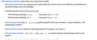
- AffineStateSpaceModel is also known as an input linear model.
- AffineStateSpaceModel can represent any system where the control input occurs affinely, but still allows for advanced analysis and control design.
- The following short input forms can be used:
-
AffineStateSpaceModel[{a,b,c},x] output given by 
AffineStateSpaceModel[{a,b},x] output given by 
- AffineStateSpaceModel[{a,b,…},x,u,y,t] explicitly specifies the input variables u, output variables y, and independent variable t.
- AffineStateSpaceModel allows for operating values for the states x and inputs u.
- AffineStateSpaceModel[…,{{x1,x10},…},{{u1,u10},…},…] is used to indicate the operating values for the system. »
- In AffineStateSpaceModel[sys] the following systems can be converted:
-
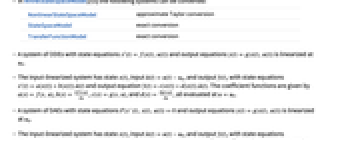
NonlinearStateSpaceModel approximate Taylor conversion StateSpaceModel exact conversion TransferFunctionModel exact conversion - A system of ODEs with state equations
 and output equations
  is linearized at
  .
. - The input-linearized system has state
 , input
  , and output
  , with state equations
  and output equation
  . The coefficient functions are given by
  ,
,  ,
,  , and
, and  , all evaluated at
  .
. - A system of DAEs with state equations
 and output equations
  is linearized at
  .
. - The input-linearized system has state
 , input
  , and output
  , with state equations
  and output equation
  . The coefficient functions are given by
  ,
,  ,
,  ,
,  , and
, and  , all evaluated at
  and
and  .
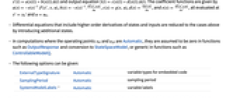
. - Differential equations that include higher-order derivatives of states and inputs are reduced to the cases above by introducing additional states.
- In computations where the operating points xi0 and uj0 are Automatic, they are assumed to be zero in functions such as OutputResponse and conversion to StateSpaceModel, or generic in functions such as ControllableModelQ.
- The following options can be given:
-
ExternalTypeSignature Automatic variable types for embedded code SamplingPeriod Automatic sampling period SystemsModelLabels Automatic variable labels - AffineStateSpaceModel can be used in functions such as OutputResponse and SystemsModelSeriesConnect.
Examples
open allclose allBasic Examples (1)
Scope (27)
Basic Uses (5)
A system with 3 states ![]() , 1 input, and 1 output:
, 1 input, and 1 output:
The response for a unit-step input:
A system with 2 inputs and 1 output:
A system with 1 input and 2 outputs:
Taylor linearize to obtain a StateSpaceModel:
Specify operating values for the states:
The state trajectories for a unit-step input:
Explicitly specify the input, output, and independent variables:
System Conversions (6)
The affine representation of a StateSpaceModel:
Specify the desired state variable names:
The affine representation of a TransferFunctionModel:
The Taylor input-linearization of a NonlinearStateSpaceModel:
The affine model of a set of ODEs:
Any nonlinear input variables in an ODE are linearized:
Affine models can be represented exactly as NonlinearStateSpaceModel:
Affine models are linearized when converting to linear models:
Model Manipulations (5)
In the model ![]() ,
, ![]() , the default d is zero:
, the default d is zero:
The default c is the identity mapping (which is not typeset):
Define operating value for the state by associating with each state variable:
Change the state operating value:
Change state, input, and output variables:
The new state, input, output, and (default) time variables:
Use Normal to get a complete list of model values ![]() :
:
Change the state variables to α and β:
If the optional variables are not specified, default symbols are assumed:
Operating Values (10)
States and inputs deleted using SystemsModelDelete are set to their operating values:
So are the states and inputs not extracted by SystemsModelExtract:
StateSpaceTransform computes the operating values of the new states if the old were specified:
By default, the simulation functions assume the operating values as the initial values:
StateSpaceModel linearizes about the operating values:
Operating values are preserved in the conversion to NonlinearStateSpaceModel:
FullInformationOutputRegulator linearizes about the operating values to compute the gains ![]() :
:
Compute the gains from the linearized subsystem:
If an operating value ![]() is given, ControllableModelQ tests controllability from
is given, ControllableModelQ tests controllability from ![]() :
:
The system is controllable from a generic point:
ControllableDecomposition behaves similarly:
If an operating value ![]() is given, ObservableModelQ tests observability at
is given, ObservableModelQ tests observability at ![]() :
:
The system is observable at a generic point:
ObservableDecomposition behaves similarly:
FeedbackLinearize linearizes at the operating value:
By default, it linearizes at the origin, which could lead to issues in some cases:
Options (2)
Applications (18)
Mechanical Systems (9)
Model a pendulum from Newton's equations for rotational motion ![]() (torque equals inertia times angular acceleration):
(torque equals inertia times angular acceleration):
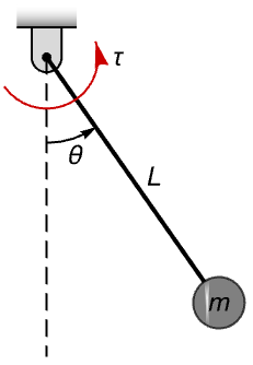
The equations are affine in the input ![]() for the applied torque:
for the applied torque:
Model a spherical pendulum below from its Lagrangian ![]() and generalized coordinates
and generalized coordinates ![]() and
and ![]() :
:
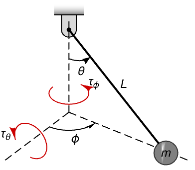
The equations of motion with generalized force ![]() are given by
are given by ![]() :
:
The equations are affine and exactly represented in AffineStateSpaceModel:
Model a double pendulum from its Hamiltonian ![]() , where
, where ![]() are generalized coordinates,
are generalized coordinates, ![]() generalized momentum, and
generalized momentum, and ![]() its Lagrangian:
its Lagrangian:
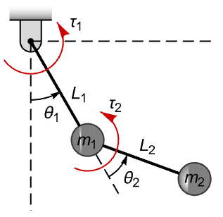
The equations of motion ![]() and
and ![]() for torque input
for torque input ![]() :
:
The equations are affine in the torque inputs ![]() :
:
Model an inverted pendulum on a cart and design a linear stabilizing controller:
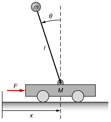
Using Lagrangian modeling with generalized coordinates ![]() and input
and input ![]() :
:
Design a controller using the linearized system:
Evaluate performance for a closed-loop system with an initial pendulum angle of 40°:
Model a ball balancing on a beam. Find whether all the internal states can be observed from the beam angle ![]() alone:
alone:
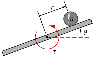
Use generalized coordinates ![]() and input
and input ![]() (torque):
(torque):
The states ![]() ,
, ![]() , and
, and ![]() can be estimated from the measurement of
can be estimated from the measurement of ![]() :
:
Model the kinematics of a car with control inputs being drive velocity and steering angle rate. Show that the car can be controlled for sideways motion by using a combination of the control inputs:
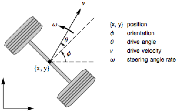
Drive velocity ![]() and steering angle rate
and steering angle rate ![]() are inputs, so there is no dynamics in the model:
are inputs, so there is no dynamics in the model:
The AffineStateSpaceModel indicates the car is controllable in all directions:
But the linearized model is not:
An example control input that combines drive and steering actions:
The state response of the model to the input:
Create the graphics of the model:
The controllability of a sleigh on a horizontal plane with the drive force ![]() and torque
and torque ![]() as inputs: »
as inputs: »
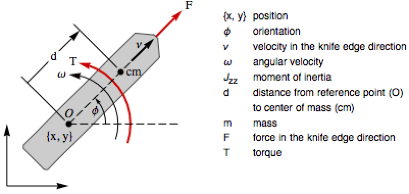
The linear system is not controllable:
The affine system is controllable using just one input:
Compute the zero dynamics of a planar vertical takeoff and landing (PVTOL) aircraft: »
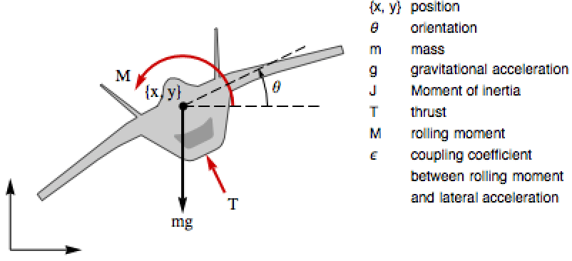
Feedback linearization reveals unstable residual dynamics:
The affine system is controllable, while its Taylor linearization is not:
Electrical Systems (4)
Model a separately excited DC motor with armature voltage, field voltage, and load torque as inputs, and see the effect of the damping on the poles of the linear approximation: »
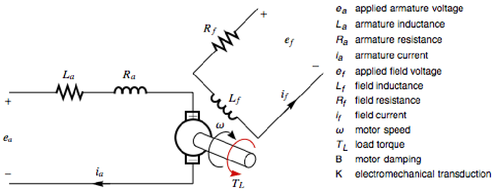
The linearized system shows the subsystems have different zeros:
The poles of the system as the damping coefficient is varied:
Model an induction motor in d-q (direct-quadrature) rotating coordinates, and use it to get a model with phase coordinates as output: »
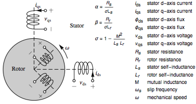
The model with states ![]() and inputs
and inputs ![]() :
:
The transformation to the phase currents and fluxes, a pure gain matrix:
The model with the phase currents and fluxes as output:
Assemble the model of a three-phase synchronous motor using the kinematic equations, which represent the relationship between the generalized coordinates and the quasi velocities, and the dynamic equations, which are obtained as Poincaré's equations. The inputs are load torque ![]() , Blondel voltages
, Blondel voltages ![]() , and winding voltage
, and winding voltage ![]() : »
: »
The generalized coordinates are the rotor angle, stator winding charges, and the field winding charge:
The quasi velocities are chosen as the angular velocity, Blondel currents, and the field current:
The kinematic relationship is ![]() :
:
The structure coefficients ![]() relative to the basis given by
relative to the basis given by ![]() :
:
The Lagrangian in terms of the quasi velocities:
The generalized force is computed as ![]() , where
, where ![]() is the Lur'e potential function:
is the Lur'e potential function:
Assemble the Poincaré equations ![]() from the Lagrangian
from the Lagrangian![]() , structure coefficients
, structure coefficients ![]() , and generalized force
, and generalized force ![]() :
:
The kinematic and Poincaré equations can be put together to obtain an affine model:
Simulate a Chua circuit for different nonlinear characteristics: »
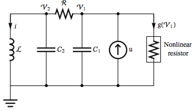
A function that plots the response of the system for different nonlinearities:
The response with a piecewise-linear nonlinearity:
Chemical Systems (5)
Compare the simulations of the affine and linear models for a reaction in a continuous fermenter: »
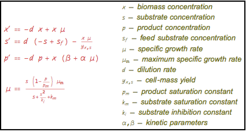
Specify the model with input ![]() , states
, states ![]() , and output
, and output ![]() , which is the productivity:
, which is the productivity:
Simulate productivity starting from some initial concentration of biomass and substrate:
The simulation shows that the nonlinear behavior is very different from the linearized behavior:
Compare the affine and linear models for a reaction in a nonisothermal continuous stirred-tank reactor (CSTR) using frequency techniques: »

Assemble the model with ![]() as input and
as input and ![]() as states:
as states:
Obtain its TransferFunctionModel by Taylor linearizing about the origin:
The BodePlot gives the frequency response of the linear system:
The gain attenuation and phase lag at frequency 1 can be obtained by reading the coordinates:
Compute the responses of the linearized and affine systems:
The plots show that the affine system does not have as much attenuation but has a greater phase lag than predicted by the linearized system:
Obtain the zero dynamics of the reaction ![]() in an isothermal CSTR: »
in an isothermal CSTR: »

The affine model with states ![]() and input
and input ![]() :
:
Its vector relative order is ![]() :
:
This implies that there is a residual system of order ![]() :
:
The zero dynamics are well behaved since ![]() :
:
Design a regulator using exact linearization to regulate the concentrations of ![]() and
and ![]() in a cyclopentenol synthesis process
in a cyclopentenol synthesis process ![]() ,
, ![]() , where
, where ![]() and
and ![]() are cylopentandiol and dicyclopentadien: »
are cylopentandiol and dicyclopentadien: »

The terms of the affine model with states ![]() and input
and input ![]() , which is the dilution rate:
, which is the dilution rate:
Determine the steady-state values:
Feedback linearize the system:
The residual dynamics are stable:
Thus a controller can be designed using the linearized dynamics:
Compare it with the response of the open-loop system:
A gas metal arc welding process can be modeled as an affine system. Design a feedback law that can maintain a specified arc length: »
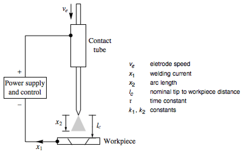
The states are ![]() and the input is the reference current
and the input is the reference current ![]() ,
, ![]() :
:
Compute a feedback law using AsymptoticOutputTracker to maintain an arc length of 1 cm:
Properties & Relations (4)
AffineStateSpaceModel converts to StateSpaceModel by linearizing states and inputs:
Conversion the other way is exact:
NonlinearStateSpaceModel converts to AffineStateSpaceModel by linearizing inputs:
Conversion the other way is exact:
Convert to TransferFunctionModel by state and input linearization:
Conversion the other way is exact:
StateSpaceTransform may produce NonlinearStateSpaceModel:
Possible Issues (1)
The input vector fields must be the columns of the input matrix:
Use Transpose to arrange them in columns:
Text
Wolfram Research (2014), AffineStateSpaceModel, Wolfram Language function, https://reference.wolfram.com/language/ref/AffineStateSpaceModel.html.
CMS
Wolfram Language. 2014. "AffineStateSpaceModel." Wolfram Language & System Documentation Center. Wolfram Research. https://reference.wolfram.com/language/ref/AffineStateSpaceModel.html.
APA
Wolfram Language. (2014). AffineStateSpaceModel. Wolfram Language & System Documentation Center. Retrieved from https://reference.wolfram.com/language/ref/AffineStateSpaceModel.html