


BodePlot
Details and Options
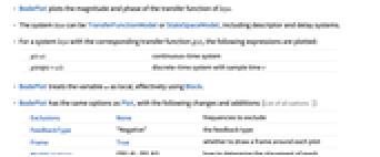
- BodePlot plots the magnitude and phase of the transfer function of lsys.
- The system lsys can be TransferFunctionModel or StateSpaceModel, including descriptor and delay systems.
- For a system lsys with the corresponding transfer function
 , the following expressions are plotted:
 -

continuous-time system 
discrete-time system with sample time 
- BodePlot treats the variable ω as local, effectively using Block.
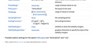
- BodePlot has the same options as Plot, with the following changes and additions: [List of all options]
-
Exclusions None frequencies to exclude FeedbackType "Negative" the feedback type Frame True whether to draw a frame around each plot MeshFunctions {{#1&},{#1&}} how to determine the placement of mesh divisions PhaseRange Automatic range of phase values to use PlotLayout "VerticalGrid" the layout to be used PlotRange {{Full,Automatic},{Full,Automatic}} range of values to include SamplingPeriod None the sampling period ScalingFunctions {{"Log10","dB"},{"Log10","Degree"}} the scaling functions StabilityMargins False whether to show the stability margins StabilityMarginsStyle Automatic graphics directives to specify the style of the stability margins - ColorData["DefaultPlotColors"] gives the default sequence of colors used by PlotStyle.
- Possible explicit settings for the option PlotLayout are "VerticalGrid" and "List".
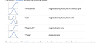
- The option PlotLayout accepts the following values:
-
"VerticalGrid" magnitude and phase plot in a vertical grid {  ,
, }
}"List" magnitude and phase plot in a list 
"Magnitude" magnitude plot only 
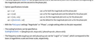
"Phase" phase plot only - The other options of BodePlot can be specified as a list of two elements, with the first element corresponding to the magnitude plot and the second to the phase plot.
- Option specifications include:
-
opt->val use val for both the magnitude and the phase plot opt->{val} use val for the magnitude plot and the default for the phase plot opt->{val1,val2} use val1 for the magnitude plot and val2 for the phase plot opt->{Automatic,val} use the default for the magnitude plot and val for the phase plot - With the PlotLayout settings "Magnitude" or "Phase", a single setting refers to the plot requested.
- The scaling functions can be specified as ScalingFunctions->{{magfreqscale,magscale},{phasefreqscale,phasescale}}.
- The frequency scales magfreqscale and phasefreqscale can be "Log10" or "Linear", which correspond to the base-10 logarithmic scale and linear scale, respectively.
- The magnitude scale magscale can be "dB" or "Absolute", which correspond to the decibel and absolute values of the magnitude, respectively.
- The phase scale phasescale can be "Degree" or "Radian".
-
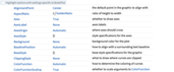
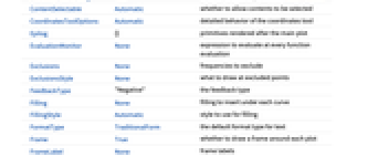
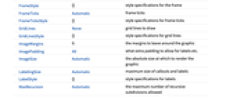
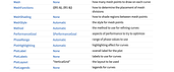
AlignmentPoint Center the default point in the graphic to align with AspectRatio 1/GoldenRatio ratio of height to width Axes True whether to draw axes AxesLabel None axes labels AxesOrigin Automatic where axes should cross AxesStyle {} style specifications for the axes Background None background color for the plot BaselinePosition Automatic how to align with a surrounding text baseline BaseStyle {} base style specifications for the graphic ClippingStyle None what to draw where curves are clipped ColorFunction Automatic how to determine the coloring of curves ColorFunctionScaling True whether to scale arguments to ColorFunction ContentSelectable Automatic whether to allow contents to be selected CoordinatesToolOptions Automatic detailed behavior of the coordinates tool Epilog {} primitives rendered after the main plot EvaluationMonitor None expression to evaluate at every function evaluation Exclusions None frequencies to exclude ExclusionsStyle None what to draw at excluded points FeedbackType "Negative" the feedback type Filling None filling to insert under each curve FillingStyle Automatic style to use for filling FormatType TraditionalForm the default format type for text Frame True whether to draw a frame around each plot FrameLabel None frame labels FrameStyle {} style specifications for the frame FrameTicks Automatic frame ticks FrameTicksStyle {} style specifications for frame ticks GridLines None grid lines to draw GridLinesStyle {} style specifications for grid lines ImageMargins 0. the margins to leave around the graphic ImagePadding All what extra padding to allow for labels etc. ImageSize Automatic the absolute size at which to render the graphic LabelingSize Automatic maximum size of callouts and labels LabelStyle {} style specifications for labels MaxRecursion Automatic the maximum number of recursive subdivisions allowed Mesh None how many mesh points to draw on each curve MeshFunctions {{#1&},{#1&}} how to determine the placement of mesh divisions MeshShading None how to shade regions between mesh points MeshStyle Automatic the style for mesh points Method Automatic the method to use for refining curves PerformanceGoal $PerformanceGoal aspects of performance to try to optimize PhaseRange Automatic range of phase values to use PlotHighlighting Automatic highlighting effect for curves PlotLabel None overall label for the plot PlotLabels None labels to use for curves PlotLayout "VerticalGrid" the layout to be used PlotLegends None legends for curves PlotPoints Automatic initial number of sample points PlotRange {{Full,Automatic},{Full,Automatic}} range of values to include PlotRangeClipping True whether to clip at the plot range PlotRangePadding Automatic how much to pad the range of values PlotRegion Automatic the final display region to be filled PlotStyle Automatic graphics directives to specify the style for each curve PlotTheme $PlotTheme overall theme for the plot PreserveImageOptions Automatic whether to preserve image options when displaying new versions of the same graphic Prolog {} primitives rendered before the main plot RegionFunction (True&) how to determine whether a point should be included RotateLabel True whether to rotate y labels on the frame SamplingPeriod None the sampling period ScalingFunctions {{"Log10","dB"},{"Log10","Degree"}} the scaling functions StabilityMargins False whether to show the stability margins StabilityMarginsStyle Automatic graphics directives to specify the style of the stability margins TargetUnits Automatic units to display in the plot Ticks Automatic axes ticks TicksStyle {} style specifications for axes ticks WorkingPrecision MachinePrecision the precision used in internal computations
List of all options
Examples
open all close allBasic Examples (3)
Scope (13)
Bode plot of a constant-gain system:
Bode plot of a differentiator:
Bode plot of a first-order lag:
Bode plot of a first-order lead:
Bode plot of a second-order system:
A higher-order TransferFunctionModel:
Bode plot of a time-delay system:
The Bode plot of a state-space model:
Generalizations & Extensions (1)
Options (21)
CoordinatesToolOptions (5)
To obtain coordinates, select the graphics and press the period key:
If frequency is in rad/s, obtain coordinate frequency values in hertz by dividing it by ![]() :
:
Coordinate frequency values in different units for each plot:
Frequency values in original units, magnitude in absolute units, and phase in radians:
Specify radians as both the displayed and copied value of phase:
GridLines (3)
PlotLayout (1)
PlotTheme (2)
SamplingPeriod (2)
Specify the sampling period in the system description:
Specify the sampling period in the BodePlot function:
ScalingFunctions (2)
Applications (7)
The static position error constant of a type 0 system is the magnitude at steady state:
The static velocity error constant of a type 1 system is approximately the intersection of the initial ![]() dB/decade segment (or its extension) with the 0 dB line:
dB/decade segment (or its extension) with the 0 dB line:
The square root of the static acceleration error constant of a type 2 system is approximately the intersection of the initial ![]() dB/decade segment (or its extension) with the 0 dB line:
dB/decade segment (or its extension) with the 0 dB line:
Visualize the improvement in phase margin by using a proportional-integral (PI) compensator:
Visualize the frequency response of a zero-order hold with sampling period 1:
Obtain the Bode plot with frequency in Hertz, when the Laplace variable is in radians/second:
For continuous-time systems, the same result can be obtained by scaling the Laplace variable:
The plot in Hertz for a discrete-time system with the Z-transform variable in radians/second:
Properties & Relations (1)
SingularValuePlot generalizes the Bode magnitude plot to MIMO systems:
Text
Wolfram Research (2010), BodePlot, Wolfram Language function, https://reference.wolfram.com/language/ref/BodePlot.html (updated 2014).
CMS
Wolfram Language. 2010. "BodePlot." Wolfram Language & System Documentation Center. Wolfram Research. Last Modified 2014. https://reference.wolfram.com/language/ref/BodePlot.html.
APA
Wolfram Language. (2010). BodePlot. Wolfram Language & System Documentation Center. Retrieved from https://reference.wolfram.com/language/ref/BodePlot.html