AsymptoticDSolveValue[eqn,f,xx0]
x0を中心とする f[x]について,微分方程式 eqn の漸近近似を計算する.
AsymptoticDSolveValue[{eqn1,eqn2,…},{f1,f2,…},xx0]
微分方程式系の漸近近似を計算する.
AsymptoticDSolveValue[eqn,f,x,ϵϵ0]
ϵ0を中心とするパラメータ ϵ の f[x,ϵ]の漸近近似を計算する.
AsymptoticDSolveValue[eqn,f,…,{ξ,ξ0,n}]
漸近近似を次数 n まで計算する.
AsymptoticDSolveValue

AsymptoticDSolveValue[eqn,f,xx0]
x0を中心とする f[x]について,微分方程式 eqn の漸近近似を計算する.
AsymptoticDSolveValue[{eqn1,eqn2,…},{f1,f2,…},xx0]
微分方程式系の漸近近似を計算する.
AsymptoticDSolveValue[eqn,f,x,ϵϵ0]
ϵ0を中心とするパラメータ ϵ の f[x,ϵ]の漸近近似を計算する.
AsymptoticDSolveValue[eqn,f,…,{ξ,ξ0,n}]
漸近近似を次数 n まで計算する.
詳細とオプション
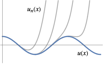
- 微分方程式の漸近近似は,漸近展開,摂動解,正則摂動,特異摂動等としても知られるものである.これらは,フロベニウス(Frobenius)級数,WKB,境界層メソッド等を計算するための特別のメソッドにも知られている.
- 漸近近似は,厳密解が求まらない問題を解くため,あるいは,計算,比較,解釈のためにより簡単な答を得るために,使われることが多い.
- AsymptoticDSolveValue[eqn,…,xx0]は,eqn の漸近展開における最大次数の項を計算する.より多くの項が指定したければSeriesTermGoalを使うとよい.
- 厳密な結果が g[x]で x0における次数 n の漸近近似が gn[x]のとき,xx0のときの結果は,AsymptoticLess[g[x]-gn[x],gn[x]-gn-1[x],xx0]または g[x]-gn[x]∈o[gn[x]-gn-1[x]]である.
- 漸近近似 gn[x]は,しばしば総和 gn[x]
αkϕk[x]として与えられる.ただし,{ϕ1[x],…,ϕn[x]}は xx0のときの漸近尺度 ϕ1[x]≻ϕ2[x]≻⋯>ϕn[x]である.結果は,xx0のとき,AsymptoticLess[g[x]-gn[x],ϕn[x],xx0]または g[x]-gn[x]∈o[ϕn[x]]である. - 次は,よく使われる漸近尺度である.
-

xx0のときのテイラー(Taylor)スケール 

xx0のときのローラン(Laurent)スケール 

x±∞のときのローランスケール 
xx0のときのピュイゾー(Puiseux)スケール - 漸近近似を表すために使われる尺度は,問題から自動的に推測される.より珍しい尺度が使われることも多い.
- 中心 x0は,任意の有限または無限の実数または複素数でよい.
- 次数 n は正の整数で,漸近解の近似次数を指定しなければならない.これは,多項式次数とは無関係である.
- u∈Vectors[n]あるいは u∈Matrices[{m,n}]という指定を使って従属変数 u がベクトル値あるいは行列値の変数であると示すことができる.u は,VectorSymbolまたはMatrixSymbolとして指定することもできる. » »
- 次は,使用可能なオプションである.
-
AccuracyGoal Automatic 目標とする絶対確度の桁数 Assumptions $Assumptions パラメータについての仮定 GenerateConditions Automatic パラメータについての条件を含む答を生成するかどうか GeneratedParameters None 生成されたパラメータの名付け方 Method Automatic 使用するメソッド PerformanceGoal $PerformanceGoal パフォーマンスのどの局面について最適化するか PrecisionGoal Automatic 目標精度の桁数 SeriesTermGoal Automatic 近似における項数 WorkingPrecision Automatic 内部計算の精度 - PerformanceGoalの可能な設定には,$PerformanceGoal,"Quality","Speed"がある."Quality"設定のとき,AsymptoticDSolveはより多くの問題を解いたりより簡単な結果を与えたりすることが多いが,より多くの時間とメモリが必要になる可能性がある.
例題
すべて開く すべて閉じる例 (3)
AsymptoticDSolveValue[{y''[x] - y[x] == 0, y[0] == 0, y'[0] == 1}, y[x], x -> 0]AsymptoticDSolveValue[{y''[x] + y[x] == 0, y[0] == 1, y'[0] == 0}, y[x], {x, 0, 10}]Plot[%, {x, 0, 3π / 2}]AsymptoticDSolveValue[{ϵ y''[x] + y'[x] + x y[x] == 0, y[0] == 0, y[1] == 1 / 2}, y[x], x, {ϵ, 0, 1}]Plot[Evaluate[Table[%, {ϵ, {1 / 30, 1 / 10, 1 / 5}}]], {x, 0, 1}]スコープ (50)
基本的な用法 (8)
常微分方程式について,x=0の周りでの次数10の級数解を計算する:
AsymptoticDSolveValue[{y''[x] + x y[x] == 0, y[0] == 0, y'[0] == 1}, y[x], {x, 0, 10}]sol = AsymptoticDSolveValue[{y'[x] - y[x] == 0, y[0] == 1}, y[x], {x, 0, 4}]Accumulateを使って近似値のリストを作る:
accum = Accumulate[List@@sol]Plot[Evaluate[accum], {x, 0, 5}, PlotLegends -> "Expressions"]AsymptoticDSolveValue[{y''[x] + 2 y[x] == 0, y[3] == 1, y'[3] == 0}, y[x], {x, 3, 10}]AsymptoticDSolveValue[y''[x] + y[x] == 0, y[x], {x, 0, 8}]AsymptoticDSolveValue[{ y'[x] + 3y[x] == 1, y[0] == 2}, y[x], {x, 0, 3}]AsymptoticDSolveValue[{ y'[x] + 3y[x] == 1, y[0] == 2}, y[x], {x, 0, 5}]AsymptoticDSolveValue[{y'[x] == z[x] + 3, z'[x] == -y[x], y[0] == 1, z[0] == 5}, {y[x], z[x]}, {x, 0, 5}]AsymptoticDSolveValue[{y'[x] + ϵ y[x] == Cos[x], y[0] == 0}, y[x], x, {ϵ, 0, 1}]AsymptoticDSolveValue[{y'[x] + ϵ y[x] == Cos[x], y[0] == 0}, y[x], x, {ϵ, 0, 2}]AsymptoticDSolveValue[{y'[x] + ϵ y[x] == Cos[x], y[0] == 0}, y[x], x, {ϵ, 0, 3}]AsymptoticDSolveValue[{ y''[x] + ϵ y'[x] + y[x] == 0, y[0] == 1, y'[0] == 0}, y[x], x, {ϵ, 0, 2}]//SimplifyPlot[Evaluate[Accumulate[CoefficientList[%, ϵ] /. {ϵ -> 1 / 100}]], {x, 0, π / 2}]通常点 (7)
通常点 x=0における一階線形常微分方程式のテイラー級数解を求める:
AsymptoticDSolveValue[{ y'[x] - x y[x] == 0, y[0] == 1}, y[x], {x, 0, 10}]Plot[Evaluate[Accumulate[List@@%]], {x, 0, 3}, PlotLegends -> "Expressions"]AsymptoticDSolveValue[{y''[x] + x y'[x] - y[x] == 0, y[0] == 1, y'[0] == 0}, y[x], {x, 0, 10}]Plot[Evaluate[Accumulate[List@@%]], {x, 0, 3}, PlotLegends -> "Expressions"]AsymptoticDSolveValue[{y'[x] + 7y[x] == E ^ x, y[0] == 1}, y[x], {x, 0, 5}]無理係数を持つ線形常微分方程式の通常点 x=0における級数解:
AsymptoticDSolveValue[{y''[x] + E ^ x y'[x] + 7 Sin[x] ^ 2 y[x] == Cos[2x], y[0] == 1, y'[0] == 5}, y[x], {x, 0, 5}]AsymptoticDSolveValue[{y''''[x] + 26 y''[x] + 25 y[x] == 0, y[0] == 1, Derivative[1][y][0] == 0, Derivative[2][y][0] == -1, Derivative[3][y][0] == 5}, y[x], {x, 0, 8}]AsymptoticDSolveValue[{y''[x] + 5y[x] == Cos[2x], y[1] == 1, y'[1] == 5}, y[x], {x, 1, 3}]AsymptoticDSolveValue[{y''[x] + 5y[x] == 0}, y[x], {x, 1, 3}]確定特異点 (5)
一階線形常微分方程式の確定特異点 x=0におけるフロベニウス級数解を求める:
AsymptoticDSolveValue[Sin[x] y'[x] + y[x] == 0, y[x], {x, 0, 7}]Plot[Evaluate[Accumulate[List@@(Expand[% /. {C[1] -> 1}])]], {x, 0, 3}, PlotLegends -> "Expressions"]AsymptoticDSolveValue[2 x ^ 2 y''[x] + 3x y'[x] - (x ^ 2 + 1)y[x] == 0, y[x], {x, 0, 5}]高次線形常微分方程式の確定特異点 x=0における級数解を求める:
AsymptoticDSolveValue[x ^ 4 y''''[x] + y[x] == 0, y[x], {x, 0, 4}]//FullSimplify(x ^ 4 y''''[x] + y[x] == 0 /. {y -> Function[{x}, Evaluate[%]]})//SimplifyAsymptoticDSolveValue[(x - 1)y''[x] + y[x] == 0, y[x], {x, 1, 2}]無理係数を持つ線形常微分方程式の確定特異点 x=0における級数解:
AsymptoticDSolveValue[Sin[x] ^ 2 * y''[x] + x y[x] == 0, y[x], {x, 0, 2}]不確定特異点 (3)
一階線形常微分方程式の不確定特異点 x=0における漸近解を求める:
AsymptoticDSolveValue[x ^ 2 y'[x] + (x ^ 2 + 1)y[x] == 0, y[x], {x, 0, 4}]Plot[Evaluate[Accumulate[List@@(Expand[% /. {C[1] -> 1}])]], {x, 0, 3}, PlotLegends -> "Expressions"]AsymptoticDSolveValue[x ^ 3 y''[x] + y[x] == 0, y[x], {x, 0, 2}]AsymptoticDSolveValue[x ^ 4 y'''[x] - 2 y'[x] + y[x] == 0, y[x], {x, 0, 2}]非線形常微分方程式 (7)
AsymptoticDSolveValue[{ y'[x] - x y[x] ^ 3 == 0, y[0] == 1}, y[x], {x, 0, 8}]Plot[Evaluate[Accumulate[List@@%]], {x, 0, 1}, PlotLegends -> "Expressions"]AsymptoticDSolveValue[{y''[x] + 2y'[x] - y[x] ^ 2 == 0, y[0] == 1, y'[0] == 0}, y, {x, 0, 6}]Plot[Evaluate[Accumulate[List@@%]], {x, 0, 3}, PlotLegends -> "Expressions"]AsymptoticDSolveValue[{y'[x] + y[x] ^ 2 == E ^ (2x), y[0] == 1}, y[x], {x, 0, 5}]AsymptoticDSolveValue[{y''[x] + y'[x] ^ 2 + 7 Sin[x] ^ 2 y[x] == Cos[2x], y[0] == 1, y'[0] == 5}, y[x], {x, 0, 5}]AsymptoticDSolveValue[{y''''[x] + y''[x] ^ 2 + 3y[x] == 0, y[0] == 1, Derivative[1][y][0] == 0, Derivative[2][y][0] == -1, Derivative[3][y][0] == 5}, y[x], {x, 0, 8}]AsymptoticDSolveValue[{y''[x] + 7y[x] ^ 2 == Cos[2x], y[1] == 1, y'[1] == 5}, y[x], {x, 1, 3}]AsymptoticDSolveValue[{y''[x] + 3y[x] ^ 3 == 0}, y[x], {x, 0, 3}]無限大における解 (4)
AsymptoticDSolveValue[x ^ 2 y'[x] + y[x] == 0, y[x], {x, ∞, 4}]Plot[Evaluate[Rest@Accumulate[List@@(% /. {C[1] -> 1})]], {x, 0, 60}, PlotLegends -> "Expressions"]線形常微分方程式の確定特異点 x=∞における級数解を求める:
AsymptoticDSolveValue[x ^ 3 y''[x] + x * y'[x] + y[x] == 0, y[x], {x, ∞, 3}]線形常微分方程式の不確定特異点 x=∞における級数解を求める:
AsymptoticDSolveValue[y''[x] - x ^ 2 y[x] == 0, y[x], {x, ∞, 2}]AsymptoticDSolveValue[{x ^ 2 y'[x] - 5y[x] ^ 2 == 0, y[∞] == 1}, y[x], {x, ∞, 4}]常微分方程式系 (8)
一階線形常微分方程式系の通常点 x=0における級数解を求める:
AsymptoticDSolveValue[{u'[x] == x v[x] + 3, v'[x] == -x u[x], u[0] == 1, v[0] == 3}, {u[x], v[x]}, {x, 0, 5}]ParametricPlot[Evaluate[%], {x, 0, 2}]AsymptoticDSolveValue[{y''[x] == z[x], z'[x] == -y[x], y[0] == 1, z[0] == 3, y'[0] == 4}, {y[x], z[x]}, {x, 0, 3}]AsymptoticDSolveValue[{y'[x] + z[x] == E ^ x, z'[x] == 5y[x] + 1, y[0] == 1, z[0] == 3}, {y[x], z[x]}, {x, 0, 5}]AsymptoticDSolveValue[{y'[x] == x z[x] + 2, z'[x] == -x y[x], y[1] == 1, z[1] == 3}, {y[x], z[x]}, {x, 1, 3}]AsymptoticDSolveValue[{y'[x] == 3 z[x], z'[x] == y[x]}, {y[x], z[x]}, {x, 1, 3}]ベクトル変数を使った通常点 x=0における常微分方程式の線形系の級数解:
m = {{0, 1}, {-1, 0}};AsymptoticDSolveValue[{y'[x] == m.y[x], y[0] == {1, 1}}, Element[y[x], Vectors[2]], {x, 0, 3}]
をVectorSymbolとして定義することもできる:
y = VectorSymbol["y", 2]AsymptoticDSolveValue[{y'[x] == m.y[x], y[0] == {1, 1}}, y[x], {x, 0, 3}]行列変数を使った通常点 x=0における常微分方程式の線形系の級数解:
m = {{0, 1}, {-1, 0}};
x0 = {{1, 2}, {3, 4}};AsymptoticDSolveValue[{y'[x] == m.y[x], y[0] == x0}, Element[y[x], Matrices[{2, 2}]], {x, 0, 3}]//MatrixForm
をMatrixSymbolとして定義することもできる:
y = MatrixSymbol["y", {2, 2}]AsymptoticDSolveValue[{y'[x] == m.y[x], y[0] == x0}, y[x], {x, 0, 3}]//MatrixFormAsymptoticDSolveValue[{Derivative[1][y1][x] == ϵ ((3 y1[x]/-6 + x) + ((1/-8 + x) + (2/-6 + x)) y2[x] + ((2/-8 + x) + (3/-6 + x)) y3[x]), Derivative[1][y2][x] == ϵ (-(4 y1[x]/-8 + x) + ((3/-8 + x) + (2/-6 + x)) y3[x]), Derivative[1][y3][x] == 0, y1[0] == 1, y2[0] == 2, y3[0] == 3}, {y1[x], y2[x], y3[x]}, x, {ϵ, 0, 2}]正則摂動 (2)
AsymptoticDSolveValue[{y''[x] - y'[x] - ϵ x y[x] == 0, y[0] == 0, y'[0] == 1}, y[x], x, {ϵ, 0, 3}]//SimplifyPlot[Evaluate[CoefficientList[%, ϵ] /. {ϵ -> 1 / 10}], {x, 0, 3}, PlotLegends -> "Expressions"]AsymptoticDSolveValue[{u''[x] + u[x] + ϵ u[x] ^ 2 == 0, u[0] == 1, u'[0] == 2}, u[x], x, {ϵ, 0, 2}]//SimplifyPlot[Evaluate[% /. {ϵ -> 1 / 100}], {x, 0, 10}]特異摂動 (3)
AsymptoticDSolveValue[{ϵ y''[x] + (x + 1) y[x] == 0, y[0] == 1, y[1] == 0}, y[x], x, {ϵ, 0, 1}]Plot[% /. {ϵ -> 1 / 500}, {x, 0, 1}]NDSolveValue[{(1 / 500) y''[x] + (x + 1) y[x] == 0, y[0] == 1, y[1] == 0}, y[x], {x, 0, 1}];Plot[%, {x, 0, 1}]AsymptoticDSolveValue[{ϵ y''[x] - (2x + 1) y[x] == 0, y[0] == 1 / 3, y[1] == 0}, y[x], x, {ϵ, 0, 2}]Plot[Table[%, {ϵ, {1 / 10, 1 / 30, 1 / 50}}]//Evaluate, {x, 0, 1}]AsymptoticDSolveValue[{y''[x] + λ (x + 1) ^ 2y[x] == 0, y[0] == 1, y[1] == 0}, y[x], x, {λ, ∞, 2}]Plot[% /. {λ -> 160}, {x, 0, 1}, WorkingPrecision -> 20]NDSolveValue[{y''[x] + 160(x + 1) ^ 2y[x] == 0, y[0] == 1, y[1] == 0}, y[x], {x, 0, 1}]Plot[%, {x, 0, 1}]非整数階常微分方程式 (3)
AsymptoticDSolveValue[{CaputoD[y[x], {x, 0.7}] + 3 y[x] == 0, y[0] == 1}, y[x], {x, 0, 5}]DSolveValueを使って同じ常微分方程式を解く:
dsol = DSolveValue[{CaputoD[y[x], {x, 0.7}] + 3 y[x] == 0, y[0] == 1}, y[x], x]asol[n_] := AsymptoticDSolveValue[{CaputoD[y[x], {x, 0.7}] + 3 y[x] == 0, y[0] == 1}, y[x], {x, 0, n}];Plot[Evaluate[{dsol, asol[5], asol[10], asol[15], asol[20]}], {x, 0, 2}, PlotLegends -> {"Exact", "n=5", "n=10", "n=15", "n=20"}]sol = AsymptoticDSolveValue[{CaputoD[y[x], {x, 1 / 2}] - x y[x] == 0, y[0] == 1}, y[x], {x, 0, 15}]eqns = {CaputoD[x1[t], {t, 0.95}] == 2x1[t] - x2[t], CaputoD[x2[t], {t, 0.95}] == 4x1[t] - 3x2[t], x1[0] == 1.2, x2[0] == 4.2};asol = AsymptoticDSolveValue[eqns, {x1, x2}, {t, 0, 15}]Plot[asol, {t, 0, 2}, PlotRange -> All]オプション (1)
アプリケーション (7)
Cosのテイラー多項式近似を計算する:
sol1 = AsymptoticDSolveValue[{y''[x] + y[x] == 0, y[0] == 1, y'[0] == 0}, y[x], {x, 0, 8}]Plot[{sol1, Cos[x]}, {x, 0, 3Pi}, PlotRange -> {-2, 5}]sol2 = AsymptoticDSolveValue[{y''[x] + y[x] == 0, y[0] == 1, y'[0] == 0}, y[x], {x, 0, 16}]Plot[{sol2, Cos[x]}, {x, 0, 3Pi}, PlotRange -> {-2, 5}]sol[n_] := AsymptoticDSolveValue[{y''[x] + y[x] == 0, y[0] == 1, y'[0] == 0}, y[x], {x, 0, n}]Plot[{sol[4], sol[8], sol[12], sol[16], sol[24], Cos[x]}//Evaluate, {x, 0, 3Pi}, PlotRange -> {-2, 5}]確定特異点 x=0付近における次数
のベッセル(Bessel)方程式を解く:
sol = AsymptoticDSolveValue[x ^ 2 y''[x] + x y'[x] + (x ^ 2 - 1 / 4)y[x] == 0, y[x], {x, 0, 24}]Plot[{(sol /. {C[1] -> 1, C[2] -> 0}), (sol /. {C[1] -> 0, C[2] -> 1})}, {x, 0, 3π}, PlotRange -> {-2, 2}]エアリー(Airy)方程式は x=∞のとき不確定特異点を持つ:
airyode = y''[x] - x y[x] == 0;sol = AsymptoticDSolveValue[airyode, y[x], {x, ∞, 3}]Infinityにおけるエアリー関数の展開と比較する:
s1 = Series[AiryAi[x], {x, ∞, 4}]//Normals2 = Series[AiryBi[x], {x, ∞, 4}]//NormalPlot[Evaluate[{AiryAi[x], AiryBi[x], (sol /. {C[1] -> 1 / (2 Sqrt[Pi]), C[2] -> 0}), (sol /. {C[1] -> 0, C[2] -> 1 / Sqrt[Pi]}) }], {x, -3, 3}, PlotLegends -> {AiryAi[x], AiryBi[x], "sol1", "sol2"},
PlotStyle -> Thickness[0.008]]ode = 3y'[x] ^ 2 + 4x y'[x] - y[x] + x ^ 2 == 0;sol = AsymptoticDSolveValue[ode, y[x], {x, 0, 4}]//Quietode /. y -> Function[{x}, Evaluate[sol]]//Simplifyodes = {u'[t] == u[t] ^ 2 / v[t] - u[t], v'[t] == u[t] ^ 2 - v[t]};StreamPlot[{u ^ 2 / v - u, u ^ 2 - v}, {u, -2, 2}, {v, -2, 2}]sol = AsymptoticDSolveValue[{odes, u[0] == a, v[0] == b}, {u[t], v[t]}, {t, 0, 5}];sol /. {a -> 1, b -> 1}eqn = {u''[x] + u[x] + ϵ u[x] ^ 3 == 0, u[0] == 3, u'[0] == 0};psol = AsymptoticDSolveValue[eqn, u[x], x, {ϵ, 0, 1}]Plot[psol /. {ϵ -> 1 / 800}, {x, 0, 20}, PlotPoints -> 100, WorkingPrecision -> 20]dsol = DSolveValue[eqn /. {ϵ -> (1/800)}, u[x], x]Plot[dsol // Evaluate, {x, 0, 20}, PlotPoints -> 100]
の大きい値についての
に対応するSturm–Liouville問題の近似固有関数を求める.より小さいパラメータ
を使ってこの問題を書き換える:
eqns = {ϵ y''[x] + (x + 1) ^ 2y[x] == 0, y[0] == A, y[1] == B};sol = FullSimplify[AsymptoticDSolveValue[eqns, y[x], x, {ϵ, 0, 1}], 0 < x < 1]定数Csc因子を無視し,
を使って,固有関数を構築する:
eigfuns = Simplify[(Sqrt[2] B Sin[(x (2 + x)/2 Sqrt[ϵ])] - A Sin[((-1 + x) (3 + x)/2 Sqrt[ϵ])]/Sqrt[1 + x]) /. {B -> 1, A -> 0, ϵ -> (9/4 n^2 π^2)}, n∈ℤ && n > 0]Plot[Table[eigfuns, {n, 1, 4}]//Evaluate, {x, 0, 1}]特性と関係 (3)
sol = AsymptoticDSolveValue[{y'[x] + y[x] == 0, y[0] == 1}, y[x], {x, 0, 8}]{y'[x] + y[x], y[0] == 1} /. y -> Function[{x}, Evaluate[sol]]DSolveValueを使って厳密解を求める:
asol = AsymptoticDSolveValue[{y'[x] - 2y[x] == 0, y[0] == 1}, y[x], {x, 0, 4}]dsol = DSolveValue[{y'[x] - 2y[x] == 0, y[0] == 1}, y[x], x]Series[%, {x, 0, 4}]//NormalNDSolveValueを使って数値解を求める:
asol = AsymptoticDSolveValue[{y'[x] + 2y[x] == 0, y[0] == 1}, y[x], {x, 0, 10}]Table[%, {x, 0, 1, 0.2}]dsol = NDSolveValue[{y'[x] + 2y[x] == 0, y[0] == 1}, y[x], {x, 0, 1}]Table[%, {x, 0, 1, 0.2}]考えられる問題 (1)
AsymptoticDSolveValue[{y''[x] + y[x] == 0, y[0] == 0, y'[0] == 1}, y[x], {x, 0, 4}]AsymptoticDSolveValue[{y''[x] + a y'[x] + y[x] == 0, y[0] == b, y'[0] == 1}, y[x], {x, 0, 4}]% /. {a -> 0, b -> 0}テクニカルノート
-
▪
- 分数階微積分学
関連するガイド
-
▪
- 漸近解析 ▪
- 方程式の解法 ▪
- 微積分 ▪
- 分数階微分積分 ▪
- 記号的なベクトル,行列,配列
テキスト
Wolfram Research (2018), AsymptoticDSolveValue, Wolfram言語関数, https://reference.wolfram.com/language/ref/AsymptoticDSolveValue.html (2026年に更新).
CMS
Wolfram Language. 2018. "AsymptoticDSolveValue." Wolfram Language & System Documentation Center. Wolfram Research. Last Modified 2026. https://reference.wolfram.com/language/ref/AsymptoticDSolveValue.html.
APA
Wolfram Language. (2018). AsymptoticDSolveValue. Wolfram Language & System Documentation Center. Retrieved from https://reference.wolfram.com/language/ref/AsymptoticDSolveValue.html
BibTeX
@misc{reference.wolfram_2026_asymptoticdsolvevalue, author="Wolfram Research", title="{AsymptoticDSolveValue}", year="2026", howpublished="\url{https://reference.wolfram.com/language/ref/AsymptoticDSolveValue.html}", note=[Accessed: 12-August-2026]}
BibLaTeX
@online{reference.wolfram_2026_asymptoticdsolvevalue, organization={Wolfram Research}, title={AsymptoticDSolveValue}, year={2026}, url={https://reference.wolfram.com/language/ref/AsymptoticDSolveValue.html}, note=[Accessed: 12-August-2026]}