ClusteringComponents[array]
给出一个数组,其中 array 中最低层的每个元素被一个表示该元素所在的连接的前景元件的整数索引所替代.
ClusteringComponents[array,n]
找到 n 个聚类.
ClusteringComponents[array,n,level]
找到 array 中指定层的聚类.
ClusteringComponents[image]
找到 image 中类似像素的最多的聚类.
ClusteringComponents[image,n]
在 image 中找到 n 个聚类.
ClusteringComponents
ClusteringComponents[array]
给出一个数组,其中 array 中最低层的每个元素被一个表示该元素所在的连接的前景元件的整数索引所替代.
ClusteringComponents[array,n]
找到 n 个聚类.
ClusteringComponents[array,n,level]
找到 array 中指定层的聚类.
ClusteringComponents[image]
找到 image 中类似像素的最多的聚类.
ClusteringComponents[image,n]
在 image 中找到 n 个聚类.
更多信息和选项
- ClusteringComponents 可用于多种数据类型,包括数字、文字、图像以及日期和时间等数据类型.
- 可以通过以下方式指定聚类的数量:
-
Automatic 自动求得聚类数量 n 精确求得 n 个聚类 UpTo[n] 求得至多 n 个聚类 - 可给出下列选项:
-
CriterionFunction Automatic 选取何种方法的准则依据 DistanceFunction Automatic 使用的距离函数 FeatureExtractor Identity 如何提取要学的特征 FeatureNames Automatic 为输入数据分配的特征名称 FeatureTypes Automatic 为输入数据分配的特征类型 Method Automatic 使用何种方法 MissingValueSynthesis Automatic 怎样合成缺失值 PerformanceGoal Automatic 优化的目标 RandomSeeding 1234 应该在伪随机发生器内部完成的种子指定方式 Weights Automatic 给予每个样本的权重 - 缺省情况下,除非指定了 DistanceFunction,ClusteringComponents 将自动对数据进行预处理.
- DistanceFunction 的设置可以是任意距离、相异度函数,或定义两个值之间的距离的函数 f.
- PerformanceGoal 的可能设置包括:
-
Automatic 自动在速度、准确度和内存间进行取舍 "Quality" 最大化分类器的准确度 "Speed" 最大化分类器的速度 - Method 的可能设置包括:
-
Automatic 自动选择方法 "Agglomerate" 单链聚类算法 "DBSCAN" 具有噪声的基于密度的空间聚类算法 "GaussianMixture" 变分高斯混合算法 "JarvisPatrick" Jarvis–Patrick 聚类算法 "KMeans" k 均值聚类算法 "KMedoids" 围绕中心点划分算法 "MeanShift" mean-shift 聚类算法 "NeighborhoodContraction" 将数据点移向高密度区域 "SpanningTree" 基于最小生成树的聚类算法 "Spectral" 谱聚类算法 - "KMeans" 和 "KMedoids" 方法只能在聚类的数量已被指定的情况下使用.
- 方法 "DBSCAN"、"GaussianMixture"、"JarvisPatrick"、"MeanShift" 和 "NeighborhoodContraction" 只能在聚类数为 Automatic 时使用.
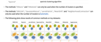
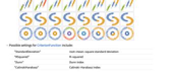
- 下图显示了玩具数据集上常用方法的结果:
- CriterionFunction 的可能设置包括:
-
"StandardDeviation" 均方根标准偏差 "RSquared" R 平方 "Dunn" Dunn 指数 "CalinskiHarabasz" Calinski–Harabasz 指数 "DaviesBouldin" Davies–Bouldin 指数 Automatic 内部指数 (internal index) - RandomSeeding 的可能设置包括:
-
Automatic 每次调用函数时都会自动重新设置种子 Inherited 使用外部种子随机数 seed 使用明确的整数或字符串作为种子
[image]范例
打开所有单元 关闭所有单元基本范例 (3)
范围 (10)
ClusteringComponents[(| | | | | |
| - | - | - | - | - |
| 1 | 2 | 2 | 2 | 1 |
| 1 | 1 | 3 | 5 | 5 |
| 1 | 1 | 5 | 5 | 5 |
| 1 | 1 | 2 | 5 | 6 |
| 1 | 1 | 4 | 5 | 6 |)] // MatrixFormClusteringComponents[[image], 5] // Colorizei = ExampleData[{"TestImage3D", "MRknee"}]seg = ClusteringComponents[i, 3];
Image3D[Colorize[seg], ClipPlanes -> {{-1, 1, 0, 12}}]ClusteringComponents[{{1, 2}, 3, {10, 11}, {12, {13}}, 14}, 2]ClusteringComponents[{{1, 2}, {3, 4}, {10, 11}, {12, 13}}, 2, 2]ClusteringComponents[{{1, 2}, {3, 4}, {10, 11}, {12, 13}}, 2, 1]ClusteringComponents[{1, 2, 2, 7, 7, 8}, UpTo[100]]ClusteringComponents[(| | | | |
| - | - | - | - |
| 1 | 1 | 7 | 7 |
| 1 | 2 | 6 | 6 |
| 1 | 6 | 5 | 5 |
| 0 | 7 | 5 | 5 |), 2]//ColorizeClusteringComponents[{{True, False, True}, {False, False, True}, {False, True, False}}, 2, 1]SeedRandom[1234];
tfdata = RandomChoice[{True, False}, {30, 3}]c = ClusteringComponents[tfdata, Automatic, 1]选项 (13)
CriterionFunction (1)
circle[r_, theta_] := {r Sin[theta], r Cos[theta]};
points = RandomVariate[MixtureDistribution[{1, 1}, {UniformDistribution[{{3 / 2, 2}, {0, 2 Pi}}], UniformDistribution[{{0, 1 / 2}, {0, 2 Pi}}]}], 1000];
data = circle@@@points;
ListPlot[data, PlotRange -> All]使用 CriterionFunction 的不同设置给出两个聚类的情况下的聚类标记结果:
assignment1 = ClusteringComponents[data, 2, 1];assignment2 = ClusteringComponents[data, 2, 1, CriterionFunction -> "CalinskiHarabasz"];cCluster1 = Pick[data, assignment1, 1];
cCluster2 = Pick[data, assignment1, 2];
ListPlot[{cCluster1, cCluster2}]dCluster1 = Pick[data, assignment2, 1];
dCluster2 = Pick[data, assignment2, 2];
ListPlot[{dCluster1, dCluster2}]DistanceFunction (1)
缺省情况下,EditDistance 被用来对字符串列表进行聚类分析:
sdata = {"GCTAT", "TAGGA", "GAATT", "CATCT", "TCAGG", "GGGGA", "TTACG", "GTCAG", "TGGAG", "GAAAA", "ATAGG", "TCCGA", "TAACT", "GTGAT", "AAGAA", "CCGTA", "GCTAA", "GCTGG", "GAGGG", "CTCAT"};ClusteringComponents[sdata, 2]使用 HammingDistance 根据相异字符的个数来进行聚类分析:
ClusteringComponents[sdata, 2, DistanceFunction -> HammingDistance]FeatureExtractor (1)
flowers = {[image], [image], [image], [image], [image], [image], [image], [image], [image], [image], [image], [image], [image], [image], [image], [image], [image], [image], [image]};ClusteringComponents[flowers, 3, 1]创建一个自定义的 FeatureExtractor 来提取特征:
fe = FeatureExtraction[flowers, (DominantColors[#, 2]&)]extractedfeatures = fe[flowers]使用 FeatureExtractor 找到新的聚类分量:
cnew = ClusteringComponents[flowers, 3, 1, FeatureExtractor -> fe]GroupBy[Transpose[{extractedfeatures, flowers, cnew}], Last -> Most]FeatureNames (1)
用 FeatureNames 命名特征,并在后面的规范中用它们的名称进行指代:
c = ClusteringComponents[{{2.3, "male"}, {4.8, "male"}, {9, "female"}, {5.2, "female"}, {1, "male"}, {10, "male"}, {5, "female"}}, Automatic, 1, FeatureNames -> {"age", "gender"}, FeatureTypes -> <|"age" -> "Numerical", "gender" -> "Nominal"|>]FeatureTypes (1)
用 FeatureTypes 强制特征的解释:
ClusteringComponents[{{2.3, "male"}, {4.8, "male"}, {9, "female"}, {5.2, "female"}, {1, "male"}, {10, "male"}, {5, "female"}}, Automatic, 1, FeatureTypes -> {"Numerical", "Nominal"}]ClusteringComponents[{{2.3, "male"}, {4.8, "male"}, {9, "female"}, {5.2, "female"}, {1, "male"}, {10, "male"}, {5, "female"}}, Automatic, 1, FeatureTypes -> {"Nominal", "Nominal"}]Method (5)
Dis = MixtureDistribution[{1, 1, 1, 1}, {
NormalDistribution[1, 1],
NormalDistribution[-5, 1],
NormalDistribution[10, 1], NormalDistribution[20, 1]}];
data = RandomVariate[Dis, 500];
Histogram[data, {-7, 25, 0.3}]使用 "GaussianMixture" 方法给出数据的聚类标记:
assignment = ClusteringComponents[data, Method -> "GaussianMixture"];clustering = Pick[data, assignment, #]& /@ DeleteDuplicates[assignment];
Histogram[clustering, {-7, 25, 0.3}]strings = DictionaryLookup["gi" ~~ __];assignment = ClusteringComponents[strings, 4, Method -> "KMedoids"];GatherBy[Transpose[{strings, assignment}], Last][[All, All, 1]]animals = [image];Table[Colorize[ClusteringComponents[animals, Method -> method]], {method, {"GaussianMixture", "NeighborhoodContraction", "MeanShift", "Spectral", "JarvisPatrick"}}]使用 "NeighborhoodContraction" 方法及其子选项给出图像的颜色聚类:
house = [image];Table[Colorize[ClusteringComponents[house, Method -> {"NeighborhoodContraction", "NeighborhoodRadius" -> t}]], {t, {0.3, 0.1, 0.05}}]用 "Spectral" 方法及其子选项给出图像的颜色聚类:
flower = [image];ClusteringComponents[flower, Method -> "Spectral"]//ColorizeMulticolumn[Table[Colorize[ClusteringComponents[flower, Method -> {"Spectral", "NeighborhoodRadius" -> t}]], {t, {0.3, 0.2, 0.1, 0.08}}], 2, Frame -> All]PerformanceGoal (1)
vectors = RandomReal[{10, 11}, {5000, 5}];AbsoluteTiming[ ClusteringComponents[vectors, Automatic, 1];]把 PerformanceGoal 设为 "Quality" 执行同样的操作:
AbsoluteTiming[ClusteringComponents[vectors, Automatic, 1, PerformanceGoal -> "Quality"];]RandomSeeding (1)
vectors = RandomReal[{10, 11}, {500, 2}];clusterings = Table[ ClusteringComponents[vectors, Automatic, 1], 5];SameQ@@clusterings通过更改 RandomSeeding 选项多次计算聚类,并比较结果:
randomclusterings = Table[ ClusteringComponents[vectors, Automatic, 1, RandomSeeding -> RandomInteger[10]], 5];SameQ@@randomclusterings应用 (2)
属性和关系 (3)
ClusteringComponents 给出聚类指数数组,而 FindClusters 返回聚类列表:
ClusteringComponents[{10, 4, 5, 6, 11}, 2]FindClusters[{10, 4, 5, 6, 11}, 2]把 ClusteringComponents 的结果转换成相似元素的分区:
list = {10, 4, 5, 6, 11};
components = ClusteringComponents[list]Map[First, GatherBy[Transpose[{list, components}], Last], {2}]FindClusters 给出同样的结果:
FindClusters[list]把 FindClusters 的结果转换成聚类指数的列表:
list = {10, 4, 5, 6, 11};
f = FindClusters[list, 2]list /. Flatten[MapIndexed[(#1 -> #2[[1]])&, f, {2}]]ClusteringComponents 给出同样的结果:
ClusteringComponents[list]可能存在的问题 (1)
当输入的子集的均值不属于输入空间时,不能使用 "KMeans" 方法:
ClusteringComponents[{{False, False, False}, {True, True, False}, {False, False, False}, {True, True, False}, {True, False, False}, {True, False, False}, {True, False, False}}, 2, 1, DistanceFunction -> (Abs[Length[#1] - Length[#2]]&), Method -> "KMeans"]文本
Wolfram Research (2010),ClusteringComponents,Wolfram 语言函数,https://reference.wolfram.com/language/ref/ClusteringComponents.html (更新于 2022 年).
CMS
Wolfram 语言. 2010. "ClusteringComponents." Wolfram 语言与系统参考资料中心. Wolfram Research. 最新版本 2022. https://reference.wolfram.com/language/ref/ClusteringComponents.html.
APA
Wolfram 语言. (2010). ClusteringComponents. Wolfram 语言与系统参考资料中心. 追溯自 https://reference.wolfram.com/language/ref/ClusteringComponents.html 年
BibTeX
@misc{reference.wolfram_2026_clusteringcomponents, author="Wolfram Research", title="{ClusteringComponents}", year="2022", howpublished="\url{https://reference.wolfram.com/language/ref/ClusteringComponents.html}", note=[Accessed: 12-August-2026]}
BibLaTeX
@online{reference.wolfram_2026_clusteringcomponents, organization={Wolfram Research}, title={ClusteringComponents}, year={2022}, url={https://reference.wolfram.com/language/ref/ClusteringComponents.html}, note=[Accessed: 12-August-2026]}