![TemplateBox[{n, z}, ExpIntegralE]](Files/ExpIntegralE.zh/42.png "TemplateBox[{n, z}, ExpIntegralE]")




ExpIntegralE
ExpIntegralE[n,z]
给出指数积分函数 ![TemplateBox[{n, z}, ExpIntegralE]](Files/ExpIntegralE.zh/1.png "TemplateBox[{n, z}, ExpIntegralE]") .
.
更多信息
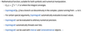
- 数学函数,适宜于符号和数值运算.
![TemplateBox[{n, z}, ExpIntegralE]=int_1^inftye^(-z t)/t^ndt](Files/ExpIntegralE.zh/2.png "TemplateBox[{n, z}, ExpIntegralE]=int_1^inftye^(-z t)/t^ndt") ,其中的积分收敛.
,其中的积分收敛.- ExpIntegralE[n,z] 在复平面 z 上有从
 到 0 的分支切割.
 - 对于某些特殊自变量,ExpIntegralE 自动计算出精确值.
- ExpIntegralE 可求任意数值精度的值.
- ExpIntegralE 自动逐项作用于列表的各个元素.
- ExpIntegralE 可与 Interval 和 CenteredInterval 对象一起使用. »
范例
打开所有单元 关闭所有单元基本范例 (5)

范围 (42)
数值计算 (5)
在高精度条件下高效计算 ExpIntegralE:
用 Interval 和 CenteredInterval 对象计算最坏情况下的区间:
或用 Around 计算一般情况下的统计区间:
或用 MatrixFunction 计算矩阵形式的 ExpIntegralE 函数:
![TemplateBox[{0, x}, ExpIntegralE]=0.5](Files/ExpIntegralE.zh/5.png "TemplateBox[{0, x}, ExpIntegralE]=0.5")
可视化 (3)
![TemplateBox[{1, z}, ExpIntegralE]](Files/ExpIntegralE.zh/6.png "TemplateBox[{1, z}, ExpIntegralE]")
![TemplateBox[{1, z}, ExpIntegralE]](Files/ExpIntegralE.zh/7.png "TemplateBox[{1, z}, ExpIntegralE]")
![TemplateBox[{{-, {7, /, 2}}, {x, +, {ⅈ, , y}}}, ExpIntegralE]](Files/ExpIntegralE.zh/8.png "TemplateBox[{{-, {7, /, 2}}, {x, +, {ⅈ, , y}}}, ExpIntegralE]")
![TemplateBox[{{-, {7, /, 2}}, {x, +, {ⅈ, , y}}}, ExpIntegralE]](Files/ExpIntegralE.zh/9.png "TemplateBox[{{-, {7, /, 2}}, {x, +, {ⅈ, , y}}}, ExpIntegralE]")
函数属性 (9)
ExpIntegralE 的实定义域:
ExpIntegralE 的复定义域:

![TemplateBox[{n, x}, ExpIntegralE]](Files/ExpIntegralE.zh/11.png "TemplateBox[{n, x}, ExpIntegralE]")
 取较小值时,ExpIntegralE 的值域可能会也可能不会更有限:
ExpIntegralE 具有镜像属性 ![TemplateBox[{0, TemplateBox[{z}, Conjugate, SyntaxForm -> SuperscriptBox]}, ExpIntegralE]=TemplateBox[{TemplateBox[{0, z}, ExpIntegralE]}, Conjugate]](Files/ExpIntegralE.zh/13.png "TemplateBox[{0, TemplateBox[{z}, Conjugate, SyntaxForm -> SuperscriptBox]}, ExpIntegralE]=TemplateBox[{TemplateBox[{0, z}, ExpIntegralE]}, Conjugate]") :
:
ExpIntegralE 不是解析函数:

![TemplateBox[{n, x}, ExpIntegralE]](Files/ExpIntegralE.zh/15.png "TemplateBox[{n, x}, ExpIntegralE]")

![TemplateBox[{n, x}, ExpIntegralE]](Files/ExpIntegralE.zh/17.png "TemplateBox[{n, x}, ExpIntegralE]")


![TemplateBox[{n, x}, ExpIntegralE]](Files/ExpIntegralE.zh/20.png "TemplateBox[{n, x}, ExpIntegralE]")
x≤0 时,ExpIntegralE 有奇点和断点:

![TemplateBox[{n, x}, ExpIntegralE]](Files/ExpIntegralE.zh/22.png "TemplateBox[{n, x}, ExpIntegralE]")


 阶导数的公式:
积分 (3)
级数展开式 (4)
![TemplateBox[{1, x}, ExpIntegralE]](Files/ExpIntegralE.zh/27.png "TemplateBox[{1, x}, ExpIntegralE]")

![TemplateBox[{0, x}, ExpIntegralE]](Files/ExpIntegralE.zh/29.png "TemplateBox[{0, x}, ExpIntegralE]")
积分变换 (3)
![TemplateBox[{0, t}, ExpIntegralE]](Files/ExpIntegralE.zh/30.png "TemplateBox[{0, t}, ExpIntegralE]")
![TemplateBox[{1, t}, ExpIntegralE]](Files/ExpIntegralE.zh/31.png "TemplateBox[{1, t}, ExpIntegralE]")
函数恒等式和化简 (4)

![TemplateBox[{1, x}, ExpIntegralE]=-TemplateBox[{{-, x}}, ExpIntegralEi]](Files/ExpIntegralE.zh/33.png "TemplateBox[{1, x}, ExpIntegralE]=-TemplateBox[{{-, x}}, ExpIntegralEi]")
函数表示 (5)
与不完全伽玛函数 Gamma 的关系:
ExpIntegralE 可以被表示为 MeijerG 的形式:
ExpIntegralE 可以被表示为 DifferentialRoot:
TraditionalForm 格式:
推广和延伸 (2)
应用 (5)
利用 ExpIntegralE 的级数展开,求水文学和电子结构计算中出现的“渗漏含水层”函数的近似(也称为 Hantush–Jacob 函数或不完全贝塞尔函数):
计算在时间  支付 1 美元的死亡保险金的预期时间值,其中
  从姜氏-梅约翰分布中提取:
求通常在保单年度开始时支付的年保险费,该保险费使得支付现金流在共  期期间的预期时间值(其中
  来自姜氏-梅约翰分布)等于净单次保险费:
属性和关系 (8)
用 FullSimplify 来化简指数积分:
用 FunctionExpand 来表示简单函数中的特殊条件:
ExpIntegralE 显示为超几何和 Meijer G 函数的一个特例:
ExpIntegralE 是一个数值函数:
ExpIntegralE 可以被表示为 DifferenceRoot:
可能存在的问题 (3)



文本
Wolfram Research (1988),ExpIntegralE,Wolfram 语言函数,https://reference.wolfram.com/language/ref/ExpIntegralE.html (更新于 2022 年).
CMS
Wolfram 语言. 1988. "ExpIntegralE." Wolfram 语言与系统参考资料中心. Wolfram Research. 最新版本 2022. https://reference.wolfram.com/language/ref/ExpIntegralE.html.
APA
Wolfram 语言. (1988). ExpIntegralE. Wolfram 语言与系统参考资料中心. 追溯自 https://reference.wolfram.com/language/ref/ExpIntegralE.html 年