Wolfram 语言与系统参考资料中心

FactorialMoment

FactorialMoment[data,r]

给出 data 的阶 r 阶乘矩 .

FactorialMoment[data,{r₁,…,r_m}]

给出 data 的阶 {r₁,…,r_m} 多元阶乘矩 .

FactorialMoment[dist,…]

给出了分布 dist 的阶乘矩.

FactorialMoment[r]

代表阶 r 形式阶乘矩.

更多信息

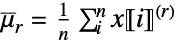
阶乘矩使用 FactorialPower[x,r] 定义，由给出.
对于标量阶 r 和作为数组的 data ：
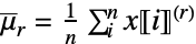
r 次阶乘幂之和 »

r 次阶乘幂列式之和 »

$x in TemplateBox[{Arrays, paclet:ref/Arrays}, RefLink, BaseStyle -> {3ColumnTableMod}][{n_(1),...,n_(k)}]$ r 次阶乘幂列式之和 »
FactorialMoment[x,r] 等价于 ArrayReduce[FactorialMoment[#,r]&,x,1].
对于向量阶 {r₁,…,r_m} 和作为数组的 data ：
第 j 列中的 r_j 次阶乘和

$x in TemplateBox[{Arrays, paclet:ref/Arrays}, RefLink, BaseStyle -> {3ColumnTableMod}][{n_(1),...,n_(k)}]$ 第 j 列中求和 r_j 次阶乘幂 »
FactorialMoment[x,{r₁,…,r_m}] 等价于 ArrayReduce[FactorialMoment[#,{r₁,…,r_m}]&,x,{{1},{2}}].
FactorialMoment 既能处理数值数据，也能处理符号数据.
data 可以有以下其他形式和解释：

	Association	值（忽略键值） »
	WeightedData	加权平均值，基于底层 EmpiricalDistribution »
	EventData	基于底层 SurvivalDistribution »
	TimeSeries, TemporalData, …	值的向量或数组（忽略时间戳） »
	Image,Image3D	RGB 通道值或灰度强度值 »
	Audio	所有通道的振幅值 »

对于分布 dist，第 r 次阶乘矩由 Expectation[x^(r),xdist] 给出. »
对于多元分布 dist，第 {r₁,…,r_m} 次阶乘矩由 Expectation[x₁^(r₁)⋯ x_m^(r_m),{x₁,…,x_m}dist] 给出. »
对于随机过程 proc，可以计算出时间 t 的切片分布的阶乘矩函数 SliceDistribution[proc,t]，因为 [t]=FactorialMoment[SliceDistribution[proc,t],r]. »
FactorialMoment[r] 可用于如 MomentConvert 和 MomentEvaluate 等函数. »

范例

打开所有单元关闭所有单元

基本范例 (2)

从数据计算阶乘矩：

使用符号数据：

计算一个离散单变量分布的二阶阶乘矩：

一个多变量分布的阶乘矩：

范围 (20)

基础用法 (5)

精确输入产生精确输出：

近似输入产生近似输出：

求 WeightedData 的阶乘矩：

求 EventData 的阶乘矩：

求 TimeSeries 的阶乘矩：

矩仅与值有关：

数组数据 (4)

对于矩阵而言，FactorialMoment 给出列向矩：

对于数组而言，FactorialMoment 给出第一层的列向矩：

数组的多元 FactorialMoment：

适用于大型数组：

当输入是 Association 时，FactorialMoment 会作用于其值：

SparseArray 数据可以像稠密数组一样使用：

图像和音频数据 (2)

RGB 图像的通道阶乘矩：

灰度图像的阶乘矩强度值：

对于音频对象，FactorialMoment 按通道工作：

分布与过程矩 (5)

单变量分布的标量阶乘矩：

多元分布的标量阶乘矩：

多元分布的联合阶乘矩：

计算符号式阶 r 的阶乘矩：

阶乘矩仅对具体阶数计算：

阶乘矩仅能做数值计算：

导出分布的阶乘矩：

数据分布：

随机过程的阶乘矩函数：

求 TemporalData 在某时刻 t=0.5 的阶乘矩：

求相应的矩函数和所有的模拟：

形式矩 (4)

形式矩的 TraditionalForm 格式：

将形式矩的组合转换为含 FactorialMoment 的表达式：

计算一个包含形式矩的分布的表达式：

对数据计算：

求包含 FactorialMoment 的一个表达式的样本估计量：

计算数据所产生的估计量：

应用 (4)

使用阶乘矩法估算分布参数：

比较数据与估计的参数分布：

从阶乘矩的序列重建概率质量函数：

求阶乘矩量生成函数 (fmgf)：

使用 fmgf 和概率生成函数的等价性：

验证求得的分布的阶乘矩与原分布匹配：

计算一些数据的移动阶乘矩：

使用长度为 .1 的窗口：

计算随机过程的路径集合的切片的阶乘矩：

选择一些切片时间：

在这些路径上绘制阶乘矩的图线：

属性和关系 (5)

阶乘矩与 FactorialPower 的期望等价：

第一阶乘矩与 Mean 等价：

FactorialMoment 可以由 Moment 通过 $mu^__r=sum_(k=1)^rTemplateBox[{r, k}, StirlingS1]mu_k$ 计算：

MomentConvert 产生相同的结果：

Moment 可由 FactorialMoment 通过 $mu_r=sum_(k=0)^rmu^__k TemplateBox[{r, k}, StirlingS2]$ 计算：

MomentConvert 产生相同的结果：

深度为的数组的多元阶乘矩的深度为：

巧妙范例 (1)

估计 30、100 和 300 个样本的 FactorialMoment 的分布：

Top

更多学习资源

技术支持

Wolfram 解决方案

Wolfram 的教育解决方案

开始

提高你的技能

与我们合作

成人教育计划

青少年教育计划

欢迎阅读

FactorialMoment

更多信息

范例

基本范例 (2)