


Fit
更多信息和选项
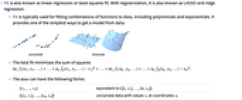
- Fit 也被称为线性回归或最小二乘拟合. 如果再加上正则化,也可被称为 LASSO 和岭回归.
- Fit 通常用于将函数组合拟合到数据,包括多项式和指数. 它提供了从数据中获取模型的最简单方法之一.
- 最佳拟合最小化平方和

. - data 可以是以下格式:
-
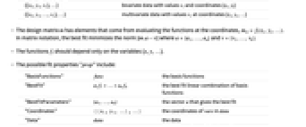
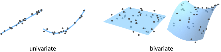
{v1,…,vn} 等同于 {{1,v1},…,{n,vn}} {{x1,v1},…,{xn,vn}} 在坐标 xi 具有值 vi 的单变量数据 {{x1,y1,v1},…} 在坐标 {xi,yi} 具有值 vi 的双变量数据 {{x1,y1,…,v1},…} 在坐标 {xi,yi,…} 具有值 vi 的多变量数据 - 设计矩阵 m 具有在坐标

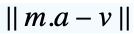
计算函数的元素. 在矩阵记法中,最佳拟合最小化范数
,其中,
且
. - 函数 fi 应该只依赖于变量 {x,y,…}.
- 可能的拟合属性 "prop" 包括:
-
"BasisFunctions 
funs 基本函数 "BestFit" 

基本函数的最佳拟合线性组合 "BestFitParameters" 

给出最佳拟合的向量 
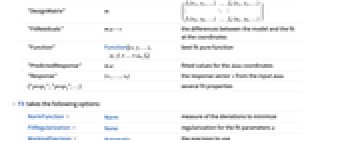
"Coordinates" {{x1,y1,…},…} data 中 vars 的坐标 "Data" data 数据 "DesignMatrix" m 

"FitResiduals" 
坐标中模型和拟合之间的差 "Function" Function[{x,y,…},a1 f1+…+an fn] 最佳拟合纯函数 "PredictedResponse" 
data 坐标的拟合值 "Response" 

来自输入 data 的响应向量 
{"prop1","prop2",…} 多个拟合属性 - Fit 接受以下选项:
-
NormFunction Norm 衡量最小化偏差 FitRegularization None 拟合参数
的正则化WorkingPrecision Automatic 使用的精度 - 当 NormFunction->normf 且 FitRegularization->rfun,Fit 找到最小化 normf[{a.f(x1,y1,…)-v1,…,a.f(xk,yk,…)-vk}] + rfun[a] 的系数向量 a.
- NormFunction 的设置可以是以下格式:
-
normf 应用于偏差的函数 normf {"Penalty", pf} 应用于偏差的每个分量的惩罚函数 pf 之和 {"HuberPenalty",α} 每个分量的 Huber 惩罚函数之和 {"DeadzoneLinearPenalty",α} 每个分量的死区线性惩罚函数之和 - FitRegularization 的设置可以是以下格式:
-
None 无正则化 rfun 用 rfun[a] 正则化 {"Tikhonov",λ} 用
正则化{"LASSO",λ} 用
正则化{"Variation",λ} 用
正则化{"TotalVariation",λ} 用
正则化{"Curvature",λ}
正则化{r1,r2,…} 用来自于 r1,… 项之和正则化 - 当 WorkingPrecision->Automatic, 作为 Fit 输入的精确数字被转换成有机器精度的近似数字.
范例
打开所有单元 关闭所有单元基本范例 (2)
data = {{0, 1}, {1, 0}, {3, 2}, {5, 4}};line = Fit[data, {1, x}, x]DesignMatrix[data, {1, x}, x]parabola = Fit[data, {1, x, x ^ 2}, x]Show[ListPlot[data, PlotStyle -> Red], Plot[{line, parabola}, {x, 0, 5}]]m = N[HilbertMatrix[4]];
v = Range[4];
a = Fit[{m, v}]范围 (2)
data = {{-Pi, 4}, {-Pi / 2, 0}, {0, 1}, {Pi / 2, -1}, {Pi, -4}};Fit[data, {Sin[x / 2], Sin[x], Sin[2 x]}, x]Fit[N[data, 24], {Sin[x / 2], Sin[x], Sin[2 x]}, x]Show[ListPlot[data], Plot[%, {x, -Pi, Pi}], PlotRange -> All]data = {{0, 0, 0}, {1, 0, 1}, {0, 1, 2}, {1, 1, 0}, {1 / 2, 1 / 2, 1}};plane = Fit[data, {1, x, y}, {x, y}]Show[Plot3D[plane, {x, 0, 1}, {y, 0, 1}, PlotStyle -> Opacity[.5], PlotRange -> {0, 2}], Graphics3D[{Red, PointSize[0.05], Map[Point, data]}]]quad = Fit[data, {1, x, y, x ^ 2, x y, y ^ 2}, {x, y}]Show[Plot3D[quad, {x, 0, 1}, {y, 0, 1}, PlotStyle -> Opacity[.5], PlotRange -> {0, 2}], Graphics3D[{Red, PointSize[0.05], Map[Point, data]}]]推广和延伸 (1)
v = {5, 4, 3, 2, 1, 0, 1, 2, 3, 4, 5};quad = Fit[v, {1, x, x ^ 2}, x]quart = Fit[v, {1, x, x ^ 2, x ^ 3, x ^ 4}, x]Show[ListPlot[v, PlotStyle -> Red], Plot[{quad, quart}, {x, 1, Length[v]}]]选项 (6)
FitRegularization (2)
data = {{0., 0.}, {0.001, 1}, {0.01, 1}};Fit[data, {1, x, x ^ 2}, x, FitRegularization -> {"Tikhonov", 1}]Fit[data, {1, x, x ^ 2}, x]这也可以用 "L2" 或 "RidgerRegression" 指代:
Fit[data, {1, x, x ^ 2}, x, FitRegularization -> {"L2", 1}]Fit[data, {1, x, x ^ 2}, x, FitRegularization -> {"RidgeRegression", 1}]LASSO (最小绝对收缩和选择算子)正则化选择最重要的基函数,并对最佳拟合参数的大小进行一些控制:
data = {{0., 0.}, {0.001, 1}, {0.01, 1}, {.1, 0}, {1, 1}};Fit[data, {1, x, x ^ 2, x ^ 3, x ^ 4}, x, FitRegularization -> {"LASSO", 1}]Fit[data, {1, x, x ^ 2, x ^ 3, x ^ 4}, x]Fit[data, {1, x, x ^ 2, x ^ 3, x ^ 4}, x, FitRegularization -> {"L1", 1}]NormFunction (3)
data = {{0, 1}, {1, 0}, {3, 2}, {5, 4}};l1 = Fit[data, {1, x}, x, NormFunction -> Function[Norm[#, 1]]]Show[ListPlot[data, PlotStyle -> PointSize[0.025]], Plot[l1, {x, 0, 5}], PlotRange -> All]l2 = Fit[data, {1, x}, x];
l∞ = Fit[data, {1, x}, x, NormFunction -> Function[Norm[#, ∞]]];
Show[ListPlot[data, PlotStyle -> PointSize[0.025]], Plot[{l1, l2, l∞}, {x, 0, 5}], PlotRange -> All]Manipulate[Plot[Evaluate[With[{q = 1 / pr}, Fit[data, {1, x}, x, NormFunction -> Function[Norm[#, q]]]]], {x, 0, 5}, PlotRange -> {-1, 4}, Epilog -> {PointSize[.025], Point[data], Text["p = " <> ToString[1 / pr], {1, 3}]}], {{pr, 1 / 2, "1/p"}, 0.0001, .9999}, SaveDefinitions -> True]使用 Huber 惩罚函数来平衡具有最小二乘的异常值的影响:
data = {{0, 1}, {1, 0}, {3, 2}, {5, 4}};hfit = Fit[data, {1, x}, x, NormFunction -> {"HuberPenalty", .1}]Show[ListPlot[data, PlotStyle -> PointSize[0.025]], Plot[hfit, {x, 0, 5}], PlotRange -> All]Manipulate[Plot[Evaluate[Fit[data, {1, x}, x, NormFunction -> {"HuberPenalty", α}]], {x, 0, 5}, PlotRange -> {-1, 4}, Epilog -> {PointSize[.025], Point[data], Text["α = " <> ToString[α], {1, 3}]}], {{α, .1}, 0.0001, 2}, SaveDefinitions -> True]data = {{0, 1}, {1, 0}, {3, 2}, {5, 4}};
fit = Fit[data, {1, x}, x, NormFunction -> Function[Norm[# Range[4]]]];
Show[ListPlot[data, PlotStyle -> PointSize[0.025]], Plot[fit, {x, 0, 5}], PlotRange -> All]应用 (6)
coord = RandomReal[{-1, 1}, 100];
data = Transpose[{coord, Sinc[10 coord]}];degree = 47;
basis = Table[ChebyshevT[k, x], {k, 0, degree}];
fit = Fit[data, basis, x];Plot[fit, {x, -1, 1}, Epilog -> Point[data]]a = N[HilbertMatrix[47]];
xexact = Table[t * (1 - t), {t, 0., 1., 1 / 46}];
b = a.xexact + 10^ - 8 RandomReal[{-1, 1}, 47];LinearSolve 找到的解有很大的项:
ListPlot[LinearSolve[a, b]]
xreg = Table[Fit[{a, b}, FitRegularization -> {"Tikhonov", 10 ^ -ll}], {ll, 0, 3, 2}];ListPlot[Prepend[xreg, xexact], PlotStyle -> PointSize[0.025]]n = 201;
m = 201;
times = Range[m];m1 = Round[m / 5]; m2 = Round[m / 4]; m3 = Round[m / 4];output = ConstantArray[0, m];
output[[m1 + Range[m2]]] = 1;
output[[m1 + m2 + Range[m3]]] = -1;
op = ListLinePlot[output]h = (1/9)(1 - .4Cos[2 times]) * .9 ^ times;hmat = ToeplitzMatrix[h, Prepend[ConstantArray[0, n - 1], h[[1]]]];没有正则化,谓词响应非常接近地匹配信号,但计算的输入有很多振荡:
{input, predicted} = Fit[{hmat, output}, {"BestFitParameters", "PredictedResponse"}];
Row[{ListLinePlot[input], ListLinePlot[{predicted, output}]}]{input, predicted} = Fit[{hmat, output}, {"BestFitParameters", "PredictedResponse"}, FitRegularization -> {"Variation", .3}];
Row[{ListLinePlot[input], ListLinePlot[{predicted, output}]}]{input, predicted} = Fit[{hmat, output}, {"BestFitParameters", "PredictedResponse"}, FitRegularization -> {{"Variation", .3}, {"Tikhonov", .01}}];
Row[{ListLinePlot[input], ListLinePlot[{predicted, output}]}]n = 4000;
times = N[Range[0, n - 1]];
original = .5 Sin[2 Pi times / n] * Sin[.01 times];
corrupted = original + RandomReal[{-.05, .05}, n];
ListLinePlot[corrupted]id = IdentityMatrix[n, SparseArray];tradeoff = Table[{smoothed, residual} = Fit[{id, corrupted}, {"BestFitParameters", "FitResiduals"}, FitRegularization -> {"Variation", 2 ^ logλ}];Tooltip[{Norm[Differences[smoothed]], Norm[residual]}, 2. ^ logλ], {logλ, -10, 20}];ListPlot[tradeoff, Joined -> True, Mesh -> All]smoothed = Fit[{id, corrupted}, "BestFitParameters", FitRegularization -> {"Variation", 100}];ListLinePlot[{corrupted, smoothed}]n = 2000;
id = IdentityMatrix[n, SparseArray];
times = Range[0, n - 1];
temp = ConstantArray[1, n / 4];
original = Join[temp, -temp, temp, -temp] + .5 Sin[2 Pi times / n];
corrupted = original + RandomReal[{-.1, .1}, n];
ListLinePlot[{corrupted, original}]smoothed = Fit[{id, corrupted}, "BestFitParameters", FitRegularization -> {"TotalVariation", 2.}];ListLinePlot[{smoothed, original}]lesssmoothed = Fit[{id, corrupted}, "BestFitParameters", FitRegularization -> {"TotalVariation", .1}];ListLinePlot[{lesssmoothed, original}]{Norm[original - smoothed], Norm[original - lesssmoothed]}使用 LASSO (L1) 正则化来找到稀疏拟合(基追踪):
σ = 0.05;
nτ = 500;
times = Subdivide[0., 1., nτ];
nω = 30;signal = (1 + .5 Sin[11 times])Sin[30 Sin[5 times]];
sdata = Transpose[{times, signal}];
ListLinePlot[sdata]Length[basis = Flatten[
Table[Exp[-(((t - τ)/σ))^2]
{1, Table[{Cos[ω t], Sin[ω t]}, {ω, Drop[Subdivide[0., 150., nω], 1]}]},
{τ, Subdivide[0., 1., nτ]}]]]AbsoluteTiming[sparseFit = Fit[sdata, basis, t, "BestFitParameters", FitRegularization -> {"LASSO", 1.}]]fitt = basis.sparseFit /. t -> times;
ListLinePlot[Transpose[{times, signal - fitt}]]一旦找到基础的重要元素,就可以通过找到最小二乘拟合这些这些元素来减少误差:
bpos = Flatten[sparseFit["NonzeroPositions"]];
sbasis = basis[[bpos]];
sbfit = Fit[sdata, sbasis, t];
ListLinePlot[Transpose[{times, signal - (sbfit /. t -> times)}], PlotRange -> All]AbsoluteTiming[sparseFit = Fit[sdata, basis, t, "BestFitParameters", FitRegularization -> {"LASSO", 0.1}]]fitt = basis.sparseFit /. t -> times;
ListLinePlot[Transpose[{times, signal - fitt}]]属性和关系 (5)
Fit 给出最佳拟合函数:
Fit[Range[10], {1, x ^ 2}, x]LinearModelFit 允许提取拟合的其他信息:
lm = LinearModelFit[Range[10], x ^ 2, x]lm["BestFit"]lm[{"RSquared", "FitResiduals", "ANOVATable"}]data = {{0, 1}, {1, 0}, {3, 2}, {5, 4}};ss[a_, b_] = Block[{x = data[[All, 1]], y = data[[All, 2]], res}, res = y - (a + b x);res.res]Minimize[ss[a, b], {a, b}]N[a + b x /. %[[2]]]这是 Fit 给出的系数:
Fit[data, {1, x}, x]精确系数可以通过使用 WorkingPrecision->Infinity 找到:
Fit[data, {1, x}, x, "BestFitParameters", WorkingPrecision -> Infinity]ss[a_, b_, c_] = Block[{x = data[[All, 1]], y = data[[All, 2]], res}, res = y - (a + b x + c x ^ 2);res.res]Minimize[ss[a, b, c], {a, b, c}]N[a + b x + c x ^ 2 /. %[[2]]]这是 Fit 给出的系数:
Fit[data, {1, x, x ^ 2}, x, "BestFitParameters", WorkingPrecision -> Infinity]当一个多项式拟合执行到足够的次数,Fit 返回插值多项式:
data = {{0, 1}, {1, 0}, {3, 2}, {5, 4}};
Fit[data, {1, x, x ^ 2, x ^ 3}, x]结果与 InterpolatingPolynomial 给出的一致:
InterpolatingPolynomial[data, x]N[Expand[%]]Fit 以变量的形式使用 TimeSeries 的时间戳:
ts1 = TemporalData[TimeSeries, {{{1.102448341846048, 6.331833897009389, 7.5843632999043455,
44.59969789743589, 98.76273258351092, 150.00729051003992, 644.7367359379259,
1724.3968817536402, 5903.697723461762, 19468.09340765025}}, {{0, 9, 1}}, 1, {"Continuous", 1},
{"Discrete", 1}, 1, {ResamplingMethod -> {"Interpolation", InterpolationOrder -> 1}}}, False,
10.1];ts1["Times"]base = {1, Exp[x], Exp[2 x], Exp[x ^ 2]};Fit[ts1, base, x]ts2 = TimeSeriesRescale[ts1, {.1, 2}]ts2["Times"]Fit[ts2, base, x]Fit[ts1["Values"], base, x]Fit 按路径作用于多条路径的 TemporalData:
Fit[TemporalData[Automatic, {{{1.102448341846048, 6.331833897009389, 7.5843632999043455,
44.59969789743589, 98.76273258351092, 150.00729051003992, 644.7367359379259,
1724.3968817536402, 5903.697723461762, 19468.09340765025},
{1.1024483418 ... 7359379259, 1724.3968817536402, 5903.697723461762,
19468.09340765025}}, {{0, 9, 1}, {0.1, 2., 0.2111111111111111}}, 2, {"Continuous", 2},
{"Discrete", 2}, 1, {ResamplingMethod -> {"Interpolation", InterpolationOrder -> 1}}}, False,
10.1], {1, Exp[x], Exp[2 x]}, x]可能存在的问题 (2)
data = Block[{r = RandomReal[100, 100]}, Transpose[{r, Exp[-(r - 50) ^ 2 / 10] + RandomReal[.1, 100]}]];
lp = ListPlot[data, PlotRange -> All]nbasis[n_Integer][x_] := Table[x ^ k, {k, 0, n}]nbasis[10][x]Table[
fit = Fit[data, nbasis[n][x], x];
Show[Plot[fit, {x, 0, 100}, PlotRange -> All], lp, PlotRange -> {-.25, 1}, PlotLabel -> "n = " <> ToString[n]],
{n, 10, 40, 10}]Fit[data, nbasis[10][x], x]Table[
fit = Fit[data, nbasis[n][(x - 50) / 50], x];
Show[Plot[fit, {x, 0, 100}, PlotRange -> All], lp, PlotRange -> {-.25, 1}, PlotLabel -> "n = " <> ToString[n]],
{n, 10, 40, 10}]k = 7;
n = 1000;
signal = Normal[SparseArray[RandomInteger[{1, n}, k] -> RandomReal[{-1, 1}, k], {n}]];
ListPlot[signal, Filling -> Axis]压缩感知包括将信号乘以
矩阵,其中
,因此只需传输长度为
的数据. 如果
足够大,具有独立相同分布的正态条目的随机矩阵将满足受限制的等距属性,并且可以非常高的概率恢复原始信号:
m = Ceiling[6 k Log[n / k]]a = RandomVariate[NormalDistribution[0, 1 / m], {m, n}];samples = a.signal;AbsoluteTiming[reconstructed = NArgMin[{Norm[x, 1], a.x == samples}, x];]Max[Abs[reconstructed - signal]]即使最小化是通过线性优化解决的,但它相对较慢,因为所有约束都是等式约束. 使用基础追踪(L1 正则化)可以更快地找到解决方案:
AbsoluteTiming[bpsol = Fit[{a, samples}, FitRegularization -> {"L1", 0.0001}]]这给出了基本要素. 要找到最佳解,求出与这些分量对应的线性方程:
basisPositions = bpsol["NonzeroPositions"];
values = LinearSolve[a[[All, Flatten[basisPositions]]], samples];
bpReconstructed = SparseArray[basisPositions -> values, {n}]Max[Abs[bpReconstructed - signal]]技术笔记
-
▪
- 处理数值数据 ▪
- 曲线拟合 ▪
- 关于内部实现的一些注释: 数值及相关函数
历史
1988年引入 (1.0) | 在以下年份被更新:2019 (12.0)
文本
Wolfram Research (1988),Fit,Wolfram 语言函数,https://reference.wolfram.com/language/ref/Fit.html (更新于 2019 年).
CMS
Wolfram 语言. 1988. "Fit." Wolfram 语言与系统参考资料中心. Wolfram Research. 最新版本 2019. https://reference.wolfram.com/language/ref/Fit.html.
APA
Wolfram 语言. (1988). Fit. Wolfram 语言与系统参考资料中心. 追溯自 https://reference.wolfram.com/language/ref/Fit.html 年
BibTeX
@misc{reference.wolfram_2026_fit, author="Wolfram Research", title="{Fit}", year="2019", howpublished="\url{https://reference.wolfram.com/language/ref/Fit.html}", note=[Accessed: 19-August-2026]}
BibLaTeX
@online{reference.wolfram_2026_fit, organization={Wolfram Research}, title={Fit}, year={2019}, url={https://reference.wolfram.com/language/ref/Fit.html}, note=[Accessed: 19-August-2026]}