

InverseBilateralZTransform
InverseBilateralZTransform[expr,z,n]
gives the inverse bilateral Z transform of expr.
InverseBilateralZTransform[expr,{z1,…,zk},{n1,…,nk}]
gives the multidimensional inverse bilateral Z transform of expr.
Details and Options
- The inverse bilateral Z transform provides the map from Fourier space back to state space, and allows one to recover the original sequence in applications of the bilateral Z transform.
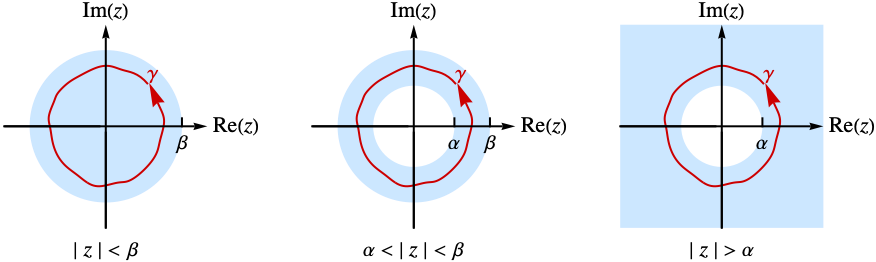
- The inverse bilateral Z transform of a function
 is given by the contour integral
  , where the integration is along a counterclockwise contour
  , lying in an annulus
 ![alpha<TemplateBox[{z}, Abs]<beta](Files/InverseBilateralZTransform.en/4.png "alpha<TemplateBox[{z}, Abs]<beta") in which the function
in which the function  is holomorphic. In some cases, the annulus of analyticity may extend to the interior or the exterior of a disk.
 - The multidimensional inverse transform is given by
 , where
  .
. - The following options can be given:
-
AccuracyGoal Automatic digits of absolute accuracy sought Assumptions $Assumptions assumptions to make about parameters GenerateConditions False whether to generate answers that involve conditions on parameters Method Automatic method to use PerformanceGoal $PerformanceGoal aspects of performance to optimize PrecisionGoal Automatic digits of precision sought WorkingPrecision Automatic the precision used in internal computations
Examples
open all close allBasic Examples (6)
Inverse bilateral Z transform of a rational function defined in an annulus:
F = ConditionalExpression[(z/(z - 1)(z - 3)), 1 < Abs[z] < 3]ComplexRegionPlot[1 < Abs[z] < 3, ...]InverseBilateralZTransform[F, z, n]DiscretePlot[%, {n, -5, 5}, PlotRange -> All]Compute the inverse transform at a single point:
InverseBilateralZTransform[ConditionalExpression[(z/(z - 1)(z - 3)), 1 < Abs[z] < 3], z, -5]N[%]InverseBilateralZTransform[ConditionalExpression[(z/(z - 1)(z - 3)), 1 < Abs[z] < 3], z, -5, WorkingPrecision -> MachinePrecision]Function defined in the exterior of a disk:
InverseBilateralZTransform[ConditionalExpression[(1/z - 1), Abs[z] > 1], z, n]DiscretePlot[%, {n, -5, 5}, PlotRange -> All]Function defined in the interior of a disk:
InverseBilateralZTransform[ConditionalExpression[(1/z - 1), Abs[z] < 1], z, n]DiscretePlot[%, {n, -5, 5}, PlotRange -> All]Function with an essential singularity at zero:
F = Exp[1 / z]ComplexPlot[F, {z, -1 - I, +1 + 1I}, Rule[...]]InverseBilateralZTransform[F, z, n]DiscretePlot[%, {n, -5, 5}, PlotRange -> All]Multivariate inverse bilateral transform:
InverseBilateralZTransform[ConditionalExpression[(z w/(z + 1)^2(w + 1)^2), Abs[z] > 1 && Abs[w] > 1], {z, w}, {n, m}]Scope (7)
InverseBilateralZTransform[ConditionalExpression[z^5, Abs[z] < Infinity], z, n]InverseBilateralZTransform[ConditionalExpression[z^-5, 0 < Abs[z]], z, n]Rational functions yield exponential and trigonometric sequences:
F = ConditionalExpression[(z^4/(z ^ 2 + 1)), Abs[z] < 1]ComplexPlot[F[[1]], {z, -2 - 2I, +2 + 2I}, Rule[...]]x[n_] = InverseBilateralZTransform[F, z, n]//FullSimplifyDiscretePlot[x[n], {n, -20, 5}]Functions involving parameters:
InverseBilateralZTransform[ConditionalExpression[(1/(z - a)(z - b)), a < Abs[z] < b], z, n]The following function defined in the interior of a circle leads to a trigonometric sequence:
InverseBilateralZTransform[ConditionalExpression[(1 - Cos[ω]z^-1/(1 - 2Cos[ω]z^-1 + z^-2)), Abs[z] < 1], z, n]FullSimplify[%, n∈Integers]If the ROC is not provided, then it is assumed to be the region containing all the function poles:
InverseBilateralZTransform[(z/(z - 1)(z ^ 2 + 1)), z, n]//FullSimplifyObtain the same result using InverseZTransform:
InverseZTransform[(z/(z - 1)(z ^ 2 + 1)), z, n]//FullSimplifyCalculate the inverse bilateral Z transform at a single point using a numerical method:
InverseBilateralZTransform[ConditionalExpression[(z/(z^2 + 4)(z^2 + 25)), 2 < Abs[z] < 5], z, 11, WorkingPrecision -> MachinePrecision]Alternatively, calculate inverse symbolically:
InverseBilateralZTransform[ConditionalExpression[(z/(z^2 + 4)(z^2 + 25)), 2 < Abs[z] < 5], z, n]Then evaluate it for a specific value of ![]() :
:
N[% /. n -> 11]For some functions, the inverse bilateral Z transform can be evaluated only numerically:
f[n_ ? NumericQ] := InverseBilateralZTransform[ConditionalExpression[(10 2^Sin[z^2]/((z ^ 2 + 1)(z - 3))), 1 < Abs[z] < 3], z, n, WorkingPrecision -> MachinePrecision]f[5]Plot the inverse bilateral Z transform using numerical values only:
DiscretePlot[Re[f[n]], {n, -10, 10}]Options (2)
Assumptions (1)
Use Assumptions to restrict the parameter domain:
InverseBilateralZTransform[ConditionalExpression[(z ^ 2 + 1/(z - 1)(z - a)), 1 < Abs[z] < 3], z, n, Assumptions -> a ≥ 3]WorkingPrecision (1)
Use WorkingPrecision to obtain a result with arbitrary precision:
F = ConditionalExpression[Exp[z ^ 2 / (z - 1)] * Sin[z], Abs[z] < 1];InverseBilateralZTransform[F, z, -7, WorkingPrecision -> MachinePrecision]InverseBilateralZTransform[F, z, -7, WorkingPrecision -> 10]InverseBilateralZTransform[F, z, -7, WorkingPrecision -> 20]Applications (2)
Define finite duration and exponentially decaying signals:
x1[n_] := 3 / 4(DiscreteDelta[n + 1] + DiscreteDelta[n] + DiscreteDelta[n - 1])
x2[n_] := 2^-Abs[n]
Plot signals in the time domain:
DiscretePlot[{x1[n], x2[n]}, {n, -5, 5}, PlotRange -> All]To find the convolution, first calculate product of the transforms:
BilateralZTransform[x1[n], n, z]BilateralZTransform[x2[n], n, z]Then, perform inversion back to the time domain:
InverseBilateralZTransform[%, z, n]//FullSimplifyPlot the convolution in the time domain:
DiscretePlot[%, {n, -5, 5}]Alternatively, find the convolution using DiscreteConvolve:
DiscreteConvolve[x1[k], x2[k], k, n]//FullSimplifyDefine a pair of infinite duration signals:
x1[n_] := n UnitStep[n]
x2[n_] := 2^nUnitStep[n - 1]
Plot the signals in the time domain:
DiscretePlot[{x1[n], x2[n]}, {n, 0, 7}]To find the convolution, first calculate the product of the transforms:
BilateralZTransform[x1[n], n, z]BilateralZTransform[x2[n], n, z]Perform inversion back to the time domain:
InverseBilateralZTransform[%, z, n]Plot the convolution in the time domain:
DiscretePlot[%, {n, 0, 6}]Alternatively, find the convolution using DiscreteConvolve:
DiscreteConvolve[x1[k], x2[k], k, n]Properties & Relations (4)
Relation to BilateralZTransform:
InverseBilateralZTransform[BilateralZTransform[x[n], n, z], z, n]InverseBilateralZTransform is closely related to InverseFourierSequenceTransform:
{InverseBilateralZTransform[ConditionalExpression[(z^2/1 / 3 + z), Abs[z] > 1 / 3], z, n], InverseFourierSequenceTransform[(z^2/1 / 3 + z) /. z -> Exp[I ω], ω, n]//Simplify}{InverseBilateralZTransform[z^-10, z, n], InverseFourierSequenceTransform[z^-10 /. z -> Exp[I ω], ω, n]}InverseBilateralZTransform[a F[z] + b G[z], z, n]InverseBilateralZTransform[ F[a * z], z, n]Possible Issues (1)
Neat Examples (1)
Create a table of basic inverse bilateral Z transforms:
CompoundExpression[...]Grid[Prepend[{#, FullSimplify[InverseBilateralZTransform[#1, z, n]]}& /@ Flist, {F[z], InverseBilateralZTransform[F[z], z, n]}], IconizedObject[«Grid options»]]//TraditionalFormText
Wolfram Research (2021), InverseBilateralZTransform, Wolfram Language function, https://reference.wolfram.com/language/ref/InverseBilateralZTransform.html.
CMS
Wolfram Language. 2021. "InverseBilateralZTransform." Wolfram Language & System Documentation Center. Wolfram Research. https://reference.wolfram.com/language/ref/InverseBilateralZTransform.html.
APA
Wolfram Language. (2021). InverseBilateralZTransform. Wolfram Language & System Documentation Center. Retrieved from https://reference.wolfram.com/language/ref/InverseBilateralZTransform.html