Using External Data
During the modeling process there are several instances where you would like to use external data. This data can be real-time inputs/outputs from sensors, recorded measurements or, in some cases, external files like CAD and images. In this tutorial, you will learn how to use external data in your models.
MODELS USED IN THIS TUTORIAL |
| CelsiusToFahrenheit FreeFloating ModelAndMeasurements |
Recorded Data
You can add recorded data like experimental measurements to your model. This is very common for data-fitting applications or for applications where physical modeling of the process is challenging. You can add your data as CombiTimeTable in Model Center, feed it as an input to your compiled models or add it to your SystemModel in the Wolfram Language.
CombiTimeTable
You can easily load custom data from your experiments using the CombiTimeTable component. This component can be found under the Modelica.Blocks.Sources package. You can specify an array of time-value pairs for the table parameter. There are also various options for time scaling, smoothness and extrapolation to adjust the output as per your needs.
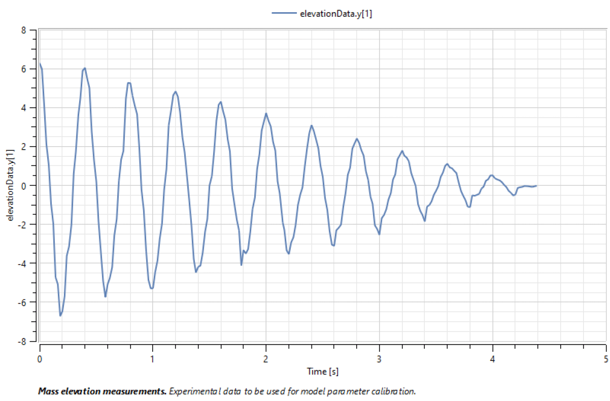
In the following, the parameters of a model are calibrated against experimental data. The measurements give the elevation of a mass suspended from a spring.
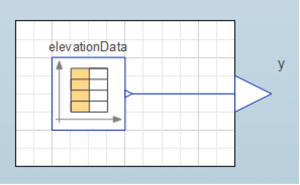
To turn the measurements into a model, a CombiTimeTable component is added to an empty model, and a connector is added for convenient access to the data later on:
The Measurements model created using components of type CombiTimeTable and RealOutput.
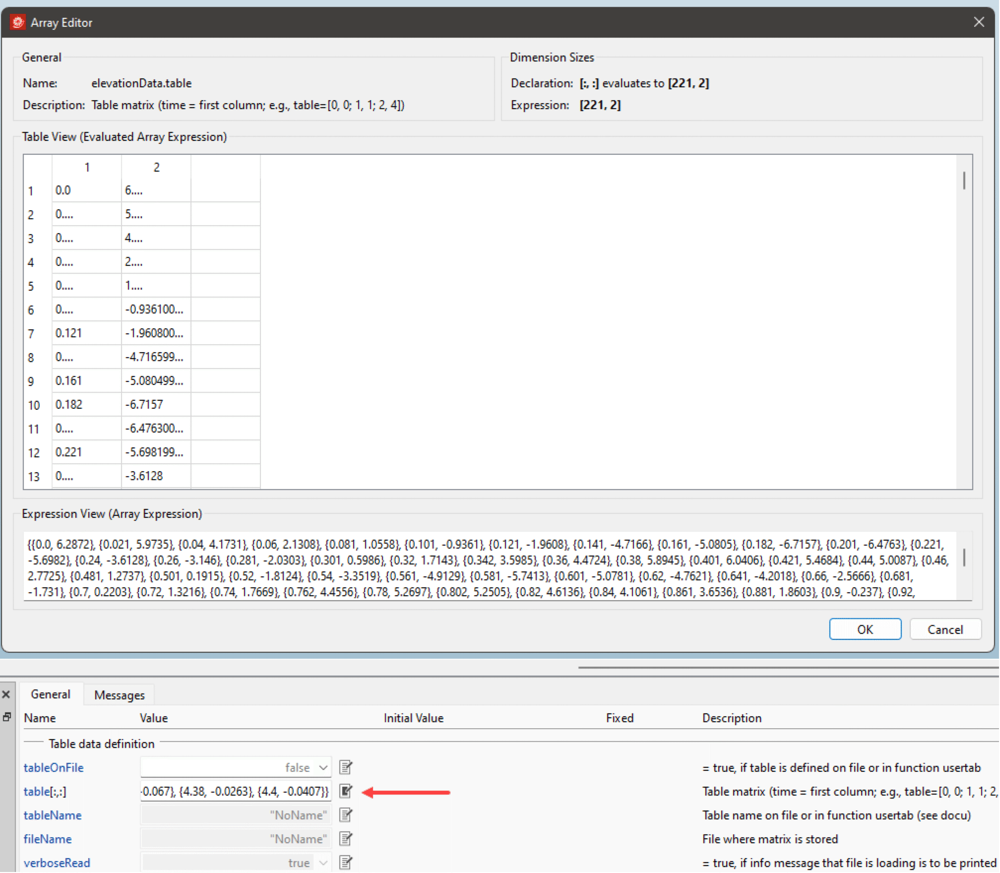
Enter measurement data by selecting the elevationData component and adding the data to its table parameter.
Adding measurement data to the table parameter of a CombiTimeTable component.
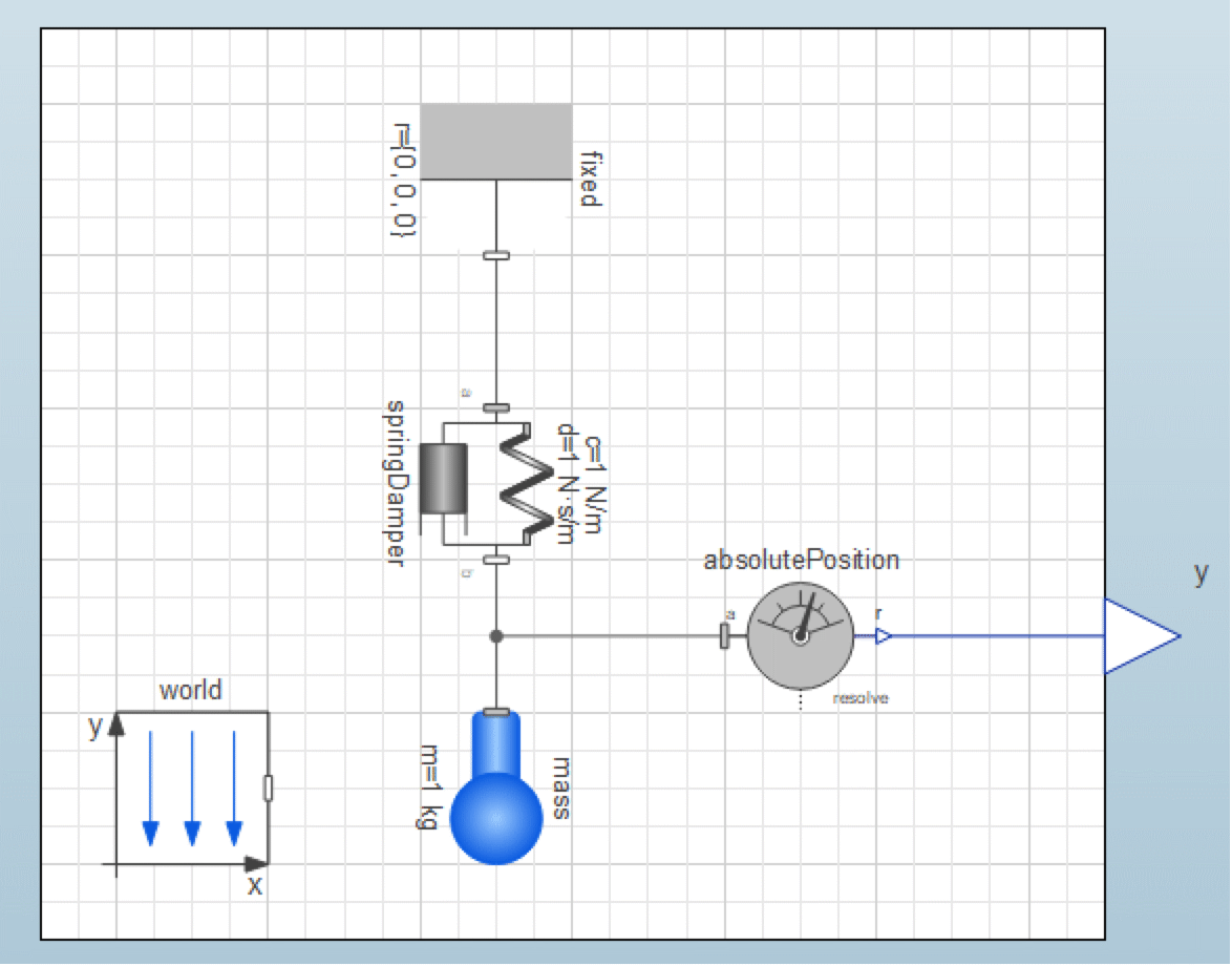
The measurements indicate that there are considerable losses in the system, so a model of the system will need to include damping in addition to the mass and and the spring:
The SpringOnMass model created using components of type World, Fixed, SpringDamperParallel, Body and AbsolutePosition.
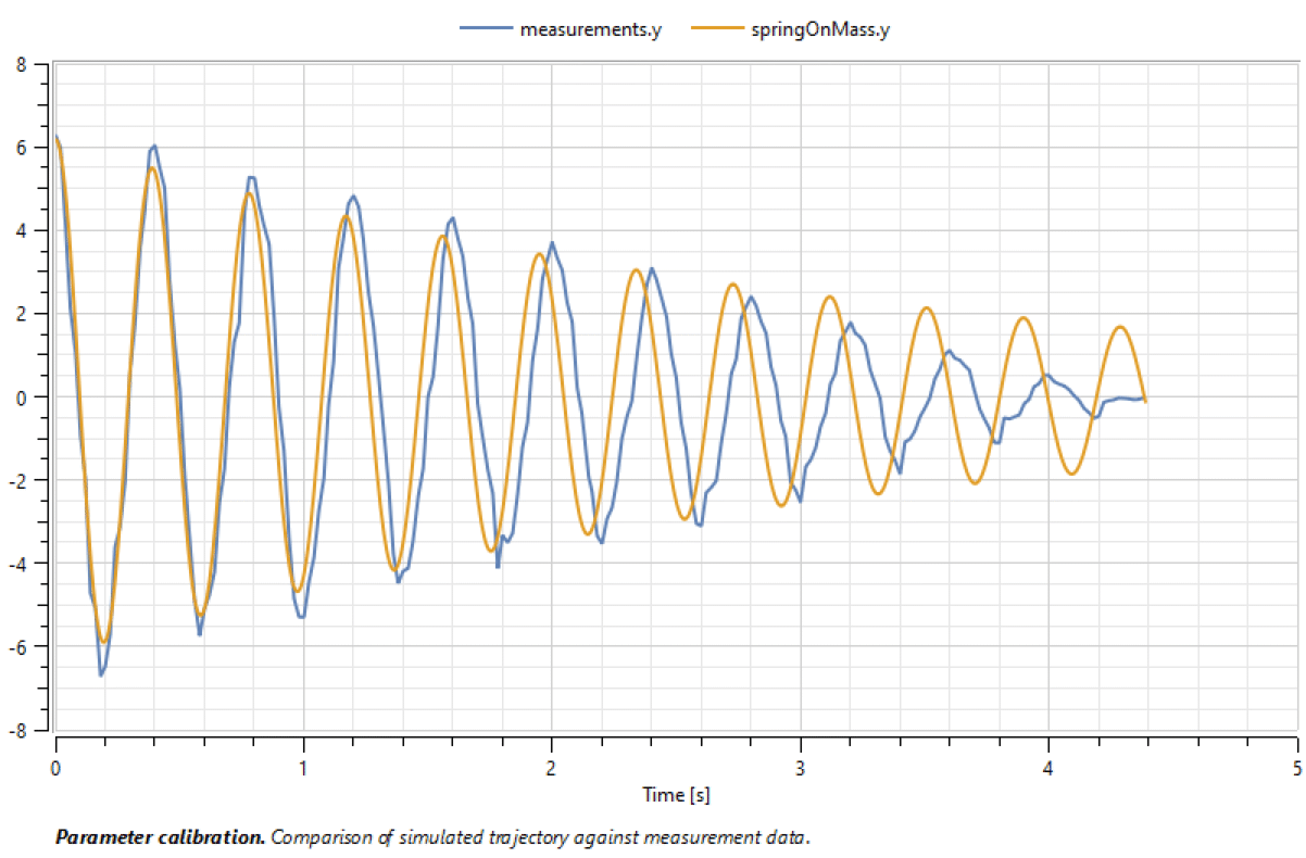
To calibrate model parameters, create a new model containing both the measurements and the SpringOnMass model. To make parameter calibration convenient, parameters selected for calibration can be lifted to the top level, as demonstrated in ModelAndMeasurements.
Calibration in progress, showing comparison of measurements to simulation using the parameter values set in the ModelAndMeasurements model.
See also: CombiTable1Dv, CombiTable2Ds, CreateDataSystemModel, Modelica CombiTimeTable
Simulation Input Data
Sometimes it is desirable to keep the recorded data separate from the model, instead of representing it as a component. An alternative approach is to provide the recorded data through a top-level input to the model, and the data is then called simulation input data.
In the following, this technique is used to feed a Celsius to Fahrenheit converter with temperature data.
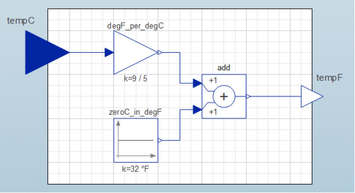
The first step is to create the model. Use components from the Modelica library and connect them in the following way (note the top-level RealInput through which temperature data in Celsius will be provided):
The CelsiusToFahrenheit model created using components of type RealInput, Gain, Constant, Add and RealOutput.
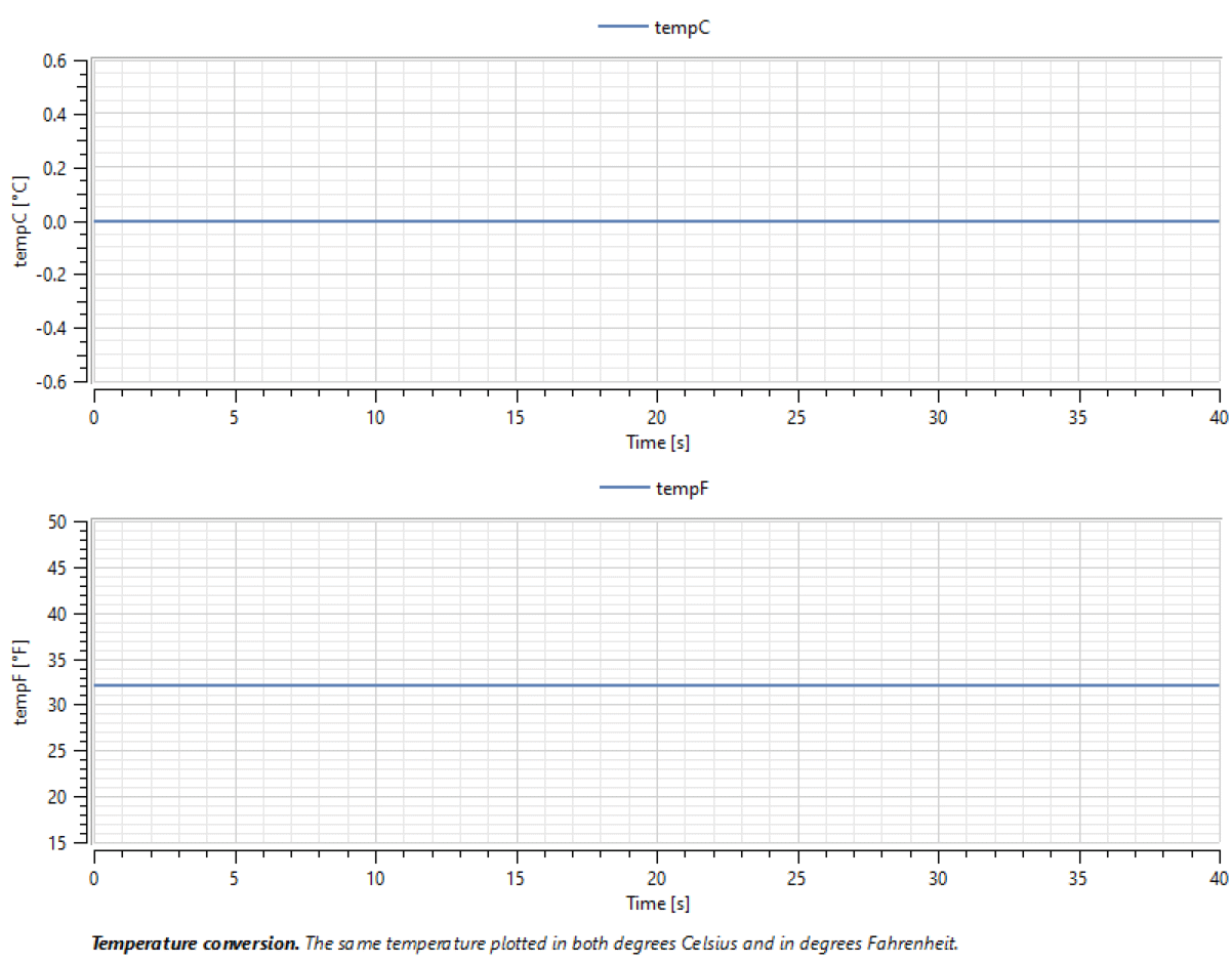
Now simulate the model. This will create a compiled version of the model, and the unconnected top-level input will be provided with a default constant zero trajectory. Plot the tempC and tempF results.
Simulating without any data fed to the top-level input.
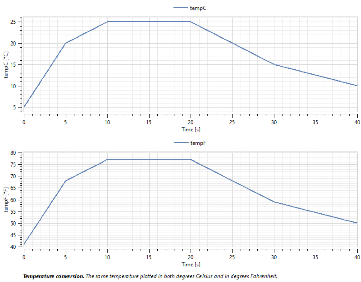
To provide simulation input data to the model, store some Celsius temperature readings in a text file using the CombiTimeTable format, where the first column is time and the second is temperature:
#1
double tempC(6, 2)
 0  5
 5 20
10 25
20 25
30 15
40 10
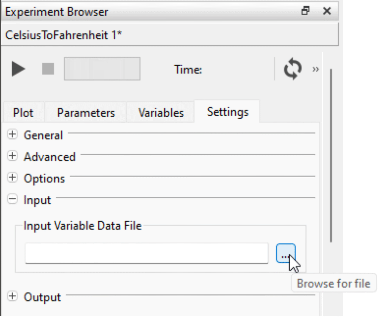
Then connect the data to the top level inputs:
Using the Input Variable Data File selector in the Experiment Browser.
Simulate again, and note how the plotted result changes:
Simulating with recorded data fed to the top-level input.
In the Wolfram Language, simulation input data can be provided with the "Inputs" option to SystemModelSimulate.
Real-Time Input/Output
Real-time connectivity has several applications. You can use it for controller-in-the-loop or hardware-in-the-loop applications. Or just plot the sensor data and study a real-world system. In this section, you will look at several ways in which you can interact with real-world applications.
OPC
The OPCUA Modelica library allows you to expand your simulation models into real-world applications. Using the open OPC Unified Architecture communication protocol, your simulations can interact with processes and hardware on a variety of different platforms. There is also an OPCClassic library for communication with OPC Classic servers, but this library is not going to be covered in this tutorial.
In the following, it will be shown how to read and write data using the OPC UA protocol.
Requirements: OPCUA library is loaded and example servers have been started according to instructions in the library documentation.
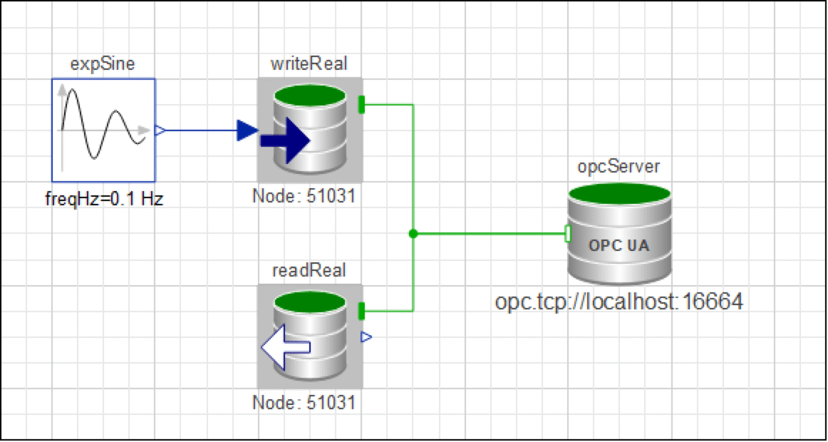
The model for demonstration will send a continuous signal from the simulation to the server and then read it back again from the server into the simulation:
The ExpSineOverOPCUA model created using components of type ExpSine, Write, Read and OPCUAServer.
The important parameters to make the communication work are nodeID, nodeIDType and nodeNamespace. They identify the node on the server that you want to read/write data. The node you specify has to exist on the server, and it has to be available for the kind of operation you want to perform, like reading or writing. Give a value to the expSine.f parameter and configure the writeReal and readReal components as follows.
Configuration of the writeReal component.
Configuration of the readReal component.
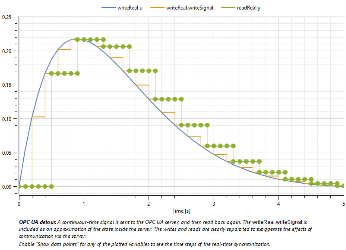
In the experiment settings, set Synchronize with real time to true and Interval length to 0.1 seconds, then simulate the model and plot the result.
Experiment settings of the ExpSineOverOPCUA model.
Simulation result showing that the detour over the OPC UA server gives an updated reading of the continuous-time signal every 0.2 seconds.
ModelPlug
The Wolfram ModelPlug library allows you to link your simulation models to the real world by the use of an Arduino board (or any other board following the Firmata protocol). ModelPlug opens up a wide variety of ways to interact with your Modelica models, for example, by using buttons, switches, input sensor information or even actuators such as motors and servos.
In the following it will be shown how a simulation can control the blinking of a LED on the Arduino board.
Requirements: ModelPlug library is loaded, the Arduino IDE and an Arduino board.
First prepare the Arduino by uploading the Firmata code to your board. The code is included with the Arduino distribution (v1.0.5 or higher) as part of the examples. Open the Arduino IDE and go to Files ▶ Examples ▶ Firmata ▶ StandardFirmata (see following figure). Open this sketch and upload it to your board.
Where to find the StandardFirmata example in the Arduino IDE.
The model in this example consists of only three components, and the rest is just to configure the components.
The BlinkLed model created using components of type BooleanPulse, DigitalOutput and Arduino.
Give a value (1 second, for example) to the booleanPulse.period parameter and configure the arduino and digitalOutput components as follows.
Configuration of the arduino component. Click the icon to the right of the the Port parameter to bring up the Serial Port Selector window.
Configuration of the digitalOutput component. The LED on the Arduino board is controlled by pin 13.
In the experiment settings, set Synchronize with real time to true and Interval length to 0.001 seconds, then simulate the model and notice how the LED is blinking.
Experiment settings of the BlinkLed model.
For further reading, see the ModelPlug GettingStarted documentation.
Graphics
Some models also need graphical assets such as a CAD object for animation or an image for icons. In this section, you will look at how you can use these types of assets.
Images
You can make your models informative by using icons. You can either create custom designs using the drawing tools or simply add an image (SVG, PNG, JPEG and BMP are supported by the Modelica Specification) to the icon view.
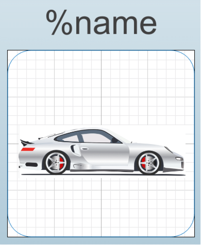
In the following, the icon of a car model is enhanced with an image. As a starting point, locate an existing image of a car or create one using a camera or a drawing tool of your choice.
Begin by creating a new model and open its Icon View. Note that the Icon View is only accessible in the Modeler user mode.
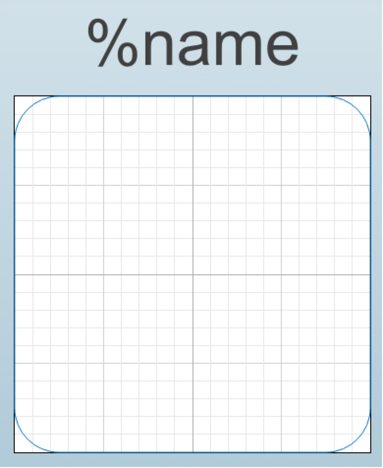
Initial icon of a model, consisting of just a rounded rectangle and a component name label.
To add the image to the icon, drag and drop it to the Icon View. Position and scale the image to occupy the desired parts of the icon. The automatically added rounded rectangle can be removed, but framing an icon is generally a good idea, especially for models with connectors.
CAD Shapes
Components from the MultiBody library allow you to attach CAD data to certain components like BodyShape, BodyBox, FixedShape and so on.
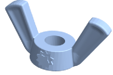
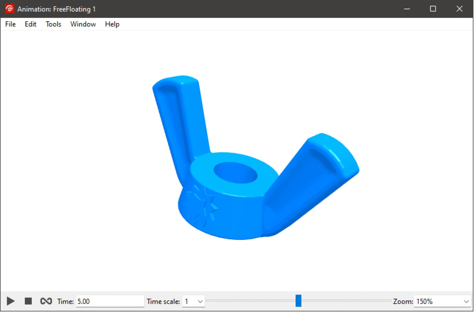
In the following, motion of a rigid body is animated using the shape of a wing nut. As a starting point, take a CAD model of a wing nut created in the Wolfram Language or any other CAD tool of your choice.
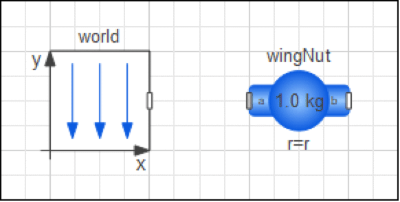
The first step is to create the model inside a package structure. Create a new package, say CADShapes, and create a model called FreeFloating inside the package. In this case, the model is essentially just a BodyShape component:
The FreeFloating model created using components of type World and BodyShape.
To model that the body is free-floating, disable gravitation by modifying the gravityType parameter of the world component. Also specify a mass for the wingNut and initialize its motion with both linear and angular velocity for a more interesting animation in the end. The bundled FreeFloating model can be used for reference.
Save the package using the Save in directory structure variant and create a new directory called Resources under the CADShapes top-level directory of the package. Store the CAD file as wingnut.stl in the Resources directory (how to properly organize external resources is beyond the scope of this tutorial).
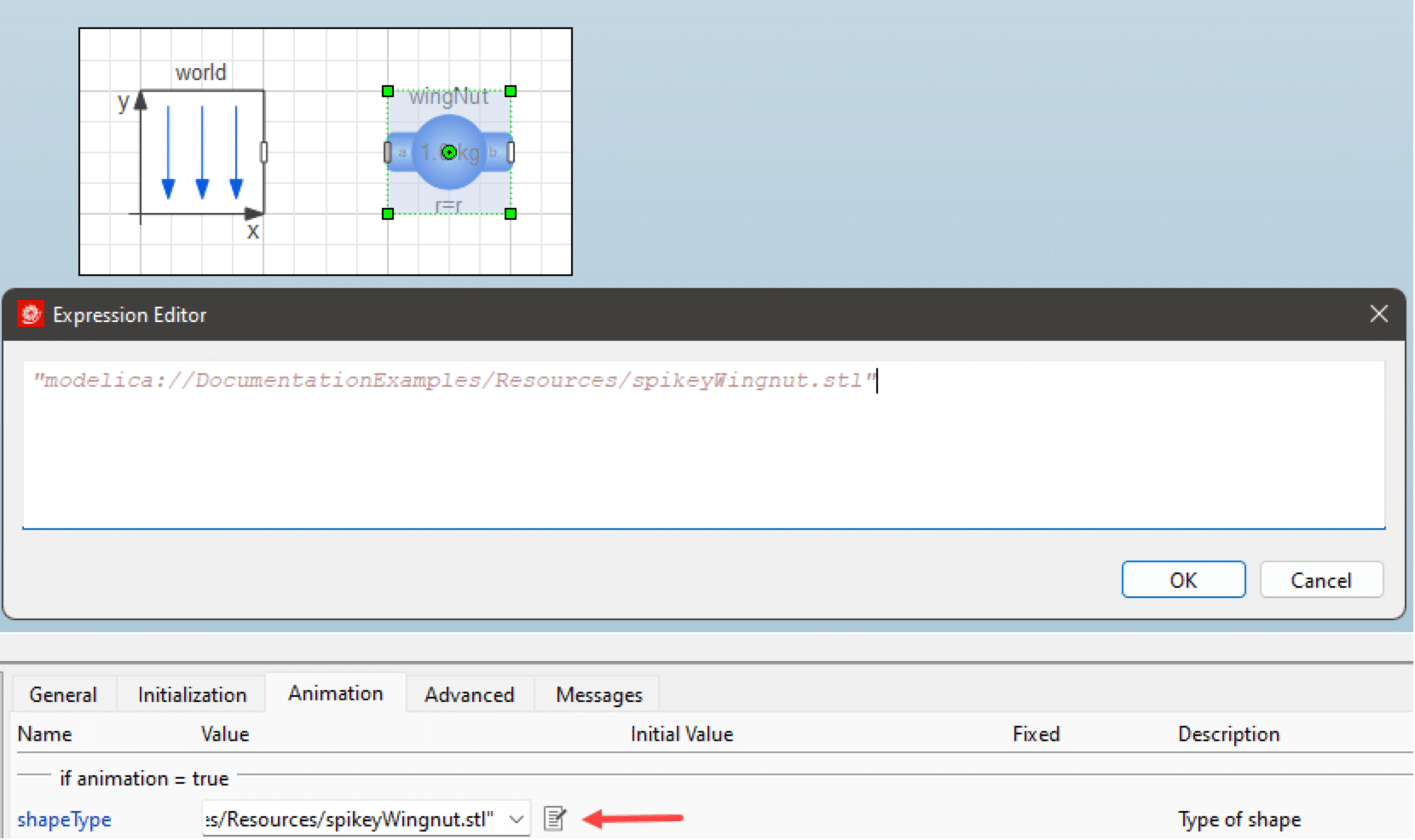
Return to Model Center and select the wingNut component in order to attach the CAD shape to it. Make the shapeType parameter listed in the Animation tab point to the CAD file using a Modelica URI:
Using a Modelica URI to specify the location of a CAD shape.
Finally simulate and play the simulation in the Animation window to see the result.
The wing nut CAD shape spinning in the Animation window.
The observant reader will have noticed that no care has been taken to correctly parameterize mass and moments of inertia of the rigid body. The Wolfram Language function CreateSystemModel can be used to automatically compute such properties based on the CAD shape and provides a robust mechanism for making sure that the properties are expressed with respect to the same coordinate system that is used for animation of the CAD shape. This technique is applied to the wing nut as well as other shapes in the blog post Simulating Zero Gravity to Demonstrate the Dzhanibekov Effect and Other Surprising Physics Models.

