


Plot3D
Plot3D[f,{x,xmin,xmax},{y,ymin,ymax}]
generates a three-dimensional plot of f as a function of x and y.
Plot3D[{f1,f2,…},{x,xmin,xmax},{y,ymin,ymax}]
plots several functions.
Plot3D[{…,w[fi],…},…]
plots fi with features defined by the symbolic wrapper w.
Plot3D[…,{x,y}∈reg]
takes variables {x,y} to be in the geometric region reg.
Details and Options
- Plot3D is also known as a surface plot or surface graph.
- Plot3D evaluates f at values of x and y in the domain being plotted over and connects the points {x,y,f[x,y]} to form a surface showing how f varies with x and y.
- It visualizes the surface
 .
. - Gaps are left at any point where the fi evaluate to anything other than real numbers.
- Plot3D treats the variables x and y as local, effectively using Block.
- Plot3D has attribute HoldAll and evaluates f only after assigning specific numerical values to x and y.
- In some cases it may be more efficient to use Evaluate to evaluate f symbolically before specific numerical values are assigned to x and y.
- The following wrappers w can be used for fi:
-
Annotation[fi,label] provide an annotation for fi Button[fi,action] evaluate action when the curve for fi is clicked Callout[fi,label] label the function with a callout Callout[fi,label,pos] place the callout at relative position pos EventHandler[fi,events] define a general event handler for fi Hyperlink[fi,uri] make the function a hyperlink Labeled[fi,label] label the function Labeled[fi,label,pos] place the label at relative position pos Legended[fi,label] identify the function in a legend PopupWindow[fi,cont] attach a popup window to the function StatusArea[fi,label] display in the status area on mouseover Style[fi,styles] show the function using the specified styles Tooltip[fi,label] attach a tooltip to the function Tooltip[fi] use functions as tooltips - Wrappers w can be applied at multiple levels:
-
w[fi] wrap fi w[{f1,…}] wrap a collection of fi w1[w2[…]] use nested wrappers - Callout, Labeled and Placed can use the following positions pos:
-
Automatic automatically placed labels Above, Below, Before, After positions around the surface {x,y} near the surface at a position {x,y} {x,y,z} at the position {x,y,z} {s,Above},{s,Below},… relative position at position s around the surface {pos,epos} epos in label placed at relative position pos of the surface - Plot3D has the same options as Graphics3D, with the following additions and changes: [List of all options]
-
Axes True whether to draw axes BoundaryStyle Automatic how to draw boundary lines for surfaces BoxRatios {1,1,0.4} bounding 3D box ratios ClippingStyle Automatic how to draw clipped parts of surfaces ColorFunction Automatic how to determine the color of surfaces ColorFunctionScaling True whether to scale arguments to ColorFunction EvaluationMonitor None expression to evaluate at every function evaluation Exclusions Automatic x, y curves to exclude ExclusionsStyle None what to draw at excluded curves Filling None filling under each surface FillingStyle Opacity[0.5] style to use for filling LabelingSize Automatic maximum size of callouts and labels MaxRecursion Automatic the maximum number of recursive subdivisions allowed Mesh Automatic how many mesh lines in each direction to draw MeshFunctions {#1&,#2&} how to determine the placement of mesh lines MeshShading None how to shade regions between mesh lines MeshStyle Automatic the style for mesh lines Method Automatic the method to use for refining surfaces NormalsFunction Automatic how to determine effective surface normals PerformanceGoal $PerformanceGoal aspects of performance to try to optimize PlotLabels None labels to use for surfaces PlotLegends None legends for surfaces PlotPoints Automatic the initial number of sample points in each direction PlotRange {Full,Full,Automatic} the range of z or other values to include PlotStyle Automatic graphics directives for the style for each surface PlotTheme $PlotTheme overall theme for the plot RegionFunction (True&) how to determine whether a point should be included ScalingFunctions None how to scale individual coordinates TextureCoordinateFunction Automatic how to determine texture coordinates TextureCoordinateScaling True whether to scale arguments to TextureCoordinateFunction WorkingPrecision MachinePrecision the precision used in internal computations - PlotStyle->None draws no surface, so effectively does not eliminate hidden surfaces.
- Plot3D initially evaluates each function at a grid of equally spaced sample points specified by PlotPoints. Then it uses an adaptive algorithm to choose additional sample points, subdividing at most MaxRecursion times.
- You should realize that with the finite number of sample points used, it is possible for Plot3D to miss features in your functions. To check your results, you should try increasing the settings for PlotPoints and MaxRecursion.
- With the setting Mesh->All, Plot3D draws mesh lines to show all subdivisions it makes.
- The default setting MeshFunctions->{#1&,#2&} draws an x, y mesh on each surface.
- The arguments supplied to functions in MeshFunctions and RegionFunction are x, y, z. Functions in ColorFunction and TextureCoordinateFunction are by default supplied with scaled versions of these arguments.
- ColorFunction, MeshFunctions, RegionFunction, and TextureCoordinateFunction are all evaluated over each surface.
- With the default settings Exclusions->Automatic and ExclusionsStyle->None, Plot3D breaks surfaces at discontinuity curves it detects. Exclusions->None joins across discontinuities.
- Possible settings for ScalingFunctions include:
-
sz scale the z axis {sx,sy} scale x and y axes {sx,sy,sz} scale x, y and z axes - Each scaling function si is either a string "scale" or {g,g-1}, where g-1 is the inverse of g.
- Plot3D returns Graphics3D[GraphicsComplex[data]].
- Themes that affect 3D surfaces include:
-
"DarkMesh" dark mesh lines 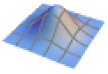
"GrayMesh" gray mesh lines 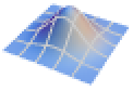
"LightMesh" light mesh lines 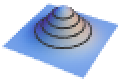
"ZMesh" vertically distributed mesh lines 
"ThickSurface" add thickness to surfaces 
"FilledSurface" add filling below surfaces

List of all options
Examples
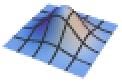
open all close allBasic Examples (4)
Plot3D[Sin[x + y ^ 2], {x, -3, 3}, {y, -2, 2}]Plot3D[{x ^ 2 + y ^ 2, -x ^ 2 - y ^ 2}, {x, -2, 2}, {y, -2, 2}, ColorFunction -> "RustTones"]Plot3D[{x ^ 2 + y ^ 2, -x ^ 2 - y ^ 2}, {x, -2, 2}, {y, -2, 2}, RegionFunction -> Function[{x, y, z}, x ^ 2 + y ^ 2 ≤ 4], BoxRatios -> Automatic]Plot functions with branch cuts:
Plot3D[Im[ArcSin[(x + I y) ^ 4]], {x, -2, 2}, {y, -2, 2}, Mesh -> None, PlotStyle -> Directive[Yellow, Specularity[White, 20], Opacity[0.8]], ExclusionsStyle -> {None, Red}]Scope (26)
Sampling (11)
More points are sampled where the function changes quickly:
Plot3D[Sin[x y], {x, 0, 3}, {y, 0, 3}, Mesh -> All]The plot range is selected automatically:
Plot3D[1 / (x ^ 2 + y ^ 2), {x, -1, 1}, {y, -1, 1}]Areas where the function becomes nonreal are excluded:
Plot3D[Sqrt[x y], {x, -1, 1}, {y, -1, 1}]The surface is split when there are discontinuities in the function:
Plot3D[Im[ArcSin[(x + I y) ^ 3]], {x, -2, 2}, {y, -2, 2}]Use PlotPoints and MaxRecursion to control adaptive sampling:
Grid[Table[Plot3D[Sin[x y], {x, 0, 4}, {y, 0, 4}, PlotPoints -> pp, MaxRecursion -> mr, Mesh -> None], {mr, {0, 1, 2}}, {pp, {5, 15}}]]Use PlotRange to focus in on areas of interest:
{Plot3D[x ^ 4 - 2x ^ 2 + y ^ 4 - 2y ^ 2 + 5, {x, -2, 2}, {y, -2, 2}], Plot3D[x ^ 4 - 2x ^ 2 + y ^ 4 - 2y ^ 2 + 1, {x, -2, 2}, {y, -2, 2}, PlotRange -> {-2, 2}, ClippingStyle -> None]}Use Exclusions to remove curves or split the resulting surface:
{Plot3D[1 / (ChebyshevU[x y - 1, 2]), {x, -5, 5}, {y, -5, 5}], Plot3D[1 / (ChebyshevU[x y - 1, 2]), {x, -5, 5}, {y, -5, 5}, Exclusions -> {x == 0, y == 0}]}Use RegionFunction to restrict the surface to a region given by inequalities:
Plot3D[Sin[x + y ^ 2], {x, -3, 3}, {y, -2, 2}, RegionFunction -> Function[{x, y, z}, 0 < x + y ^ 2 < Pi]]The domain may be specified by a region:
Plot3D[Sin[x + Cos[y]], {x, y}∈Disk[{0, 0}, 3]]The domain may be specified by a MeshRegion:
𝒟 = MeshRegion[{{0, 0}, {5, -2}, {3, 0}, {5, 2}}, Polygon[{1, 2, 3, 4}]];Plot3D[x ^ 2 + y ^ 2, {x, y}∈𝒟]Plot3D[ArcTan[x]ArcTan[y], {x, -Infinity, Infinity}, {y, -Infinity, Infinity}]Labeling and Legending (6)
Label surfaces with Labeled:
Plot3D[Labeled[Sin[x + Cos[y]], "label"], {x, -3, 3}, {y, -3, 3}]Label surfaces with PlotLabels:
Plot3D[Sin[x + Cos[y]], {x, -3, 3}, {y, -3, 3}, PlotLabels -> Sin[x + Cos[y]]]Place the label near the surface at an {x,y} value:
Plot3D[Labeled[Sin[x + Cos[y]], "label", {0, 0}], {x, -3, 3}, {y, -3, 3}]Use Callout:
Plot3D[Callout[Sin[x + Cos[y]], "label", {0, 0}], {x, -3, 3}, {y, -3, 3}, PlotRange -> All]Place a label with a specific location:
Plot3D[Callout[Sin[x + Cos[y]], "label", {2, 0, 1}], {x, -3, 3}, {y, -3, 3}, PlotRange -> All]Include legends for each surface:
Plot3D[{x ^ 2 + y ^ 2, -x ^ 2 - y ^ 2}, {x, -2, 2}, {y, -2, 2}, PlotLegends -> "Expressions"]Use Legended to provide a legend for a specific curve:
Plot3D[{x ^ 2 + y ^ 2, Legended[-x ^ 2 - y ^ 2, "surface"]}, {x, -2, 2}, {y, -2, 2}]Use Placed to change the legend location:
Plot3D[{x ^ 2 + y ^ 2, Legended[-x ^ 2 - y ^ 2, Placed["surface", Below]]}, {x, -2, 2}, {y, -2, 2}]Presentation (9)
Provide an explicit PlotStyle for the surface:
Plot3D[Sin[x + y ^ 2], {x, -2, 2}, {y, -2, 2}, PlotStyle -> Directive[Orange, Specularity[White, 20]]]Provide separate styles for different surfaces:
Plot3D[{Sin[x], Cos[x]}, {x, 0, 2Pi}, {y, 0, 2Pi}, PlotStyle -> {Red, Blue}]Plot3D[Sin[x y], {x, 0, 3}, {y, 0, 3}, AxesLabel -> {x, y}, PlotLabel -> Sin[x y]]Plot3D[Sin[x y], {x, 0, 3}, {y, 0, 3}, ColorFunction -> Function[{x, y, z}, Hue[z]]]Plot3D[Sin[x y], {x, 0, 3}, {y, 0, 3}, ColorFunction -> "SolarColors", PlotLegends -> Automatic]Use a theme with bright colors and height-based mesh lines:
Plot3D[Sin[x]Cos[y], {x, 0, 2π}, {y, 0, 2π}, PlotTheme -> "Web"]Style the areas between mesh lines:
Plot3D[Sqrt[1 - x ^ 2 - y ^ 2], {x, -1, 1}, {y, -1, 1}, Mesh -> 8, ColorFunction -> Hue, MeshShading -> {{Yellow, Orange}, {Pink, Red}}]Provide an interactive Tooltip for a surface:
Plot3D[Tooltip[Sqrt[x y]], {x, -2, 2}, {y, -2, 2}]Plot3D[Sin[x + y ^ 2], {x, -2, 2}, {y, -2, 2}, RegionFunction -> (#1 ^ 2 + #2 ^ 2 < 4&), Filling -> Bottom, FillingStyle -> Directive[Opacity[0.4], Red]]Options (103)
Background (1)
BoundaryStyle (6)
Use a black boundary around the edges of the surface:
Plot3D[Sin[x y], {x, -2, 2}, {y, -2, 2}]Use a thick boundary around the edges of the surface:
Plot3D[Sin[x y], {x, -2, 2}, {y, -2, 2}, BoundaryStyle -> Thick]Use a thick, red boundary around the edges of the surface:
Plot3D[Sin[x y], {x, -2, 2}, {y, -2, 2}, BoundaryStyle -> Directive[Red, Thick]]Plot3D[Sin[x y], {x, -2, 2}, {y, -2, 2}, BoundaryStyle -> None]BoundaryStyle applies to holes cut by RegionFunction:
Plot3D[Sin[x y], {x, -2, 2}, {y, -2, 2}, BoundaryStyle -> Thick, RegionFunction -> Function[{x, y, z}, x ^ 2 + y ^ 2 ≥ 1]]BoundaryStyle does not apply to holes cut by Exclusions:
Plot3D[Im[Sqrt[x + I y]], {x, -2, 2}, {y, -2, 2}, BoundaryStyle -> Thick]BoxRatios (2)
Automatic uses the natural scale from PlotRange:
{Plot3D[Sqrt[1 - x ^ 2 - y ^ 2], {x, 0, 1}, {y, 0, 1}], Plot3D[Sqrt[1 - x ^ 2 - y ^ 2], {x, 0, 1}, {y, 0, 1}, BoxRatios -> Automatic]}Use BoxRatios to emphasize some particular feature, in this case a saddle surface:
Plot3D[y ^ 2 - x ^ 2, {x, -4, 4}, {y, -4, 4}, MeshFunctions -> {#3&}, BoxRatios -> {1, 1, 2}]ClippingStyle (4)
Clipped regions use different surface colors by default:
Plot3D[Re[Sin[x + I y]], {x, -2Pi, 2Pi}, {y, -2Pi, 2Pi}]Plot3D[Re[Sin[x + I y]], {x, -2Pi, 2Pi}, {y, -2Pi, 2Pi}, ClippingStyle -> None]Make clipped regions partially transparent:
Plot3D[Re[Sin[x + I y]], {x, -2Pi, 2Pi}, {y, -2Pi, 2Pi}, ClippingStyle -> Opacity[0.5]]Color clipped regions red at the bottom and blue at the top:
Plot3D[Re[Sin[x + I y]], {x, -2Pi, 2Pi}, {y, -2Pi, 2Pi}, ClippingStyle -> {Red, Blue}]ColorFunction (6)
Color according to the ![]() and
and ![]() coordinates:
coordinates:
Plot3D[Sin[x y], {x, 0, 3}, {y, 0, 3}, ColorFunction -> Function[{x, y, z}, RGBColor[x, y, 0.]]]Plot3D[x / Exp[x ^ 2 + y ^ 2], {x, -2, 2}, {y, -2, 2}, ColorFunction -> Function[{x, y, z}, Hue[.65(1 - z)]]]Use ColorData for predefined color gradients:
Plot3D[x / Exp[x ^ 2 + y ^ 2], {x, -2, 2}, {y, -2, 2}, ColorFunction -> (ColorData["DarkRainbow"][#3]&)]Named color gradients color in the ![]() direction:
direction:
Plot3D[x / Exp[x ^ 2 + y ^ 2], {x, -2, 2}, {y, -2, 2}, ColorFunction -> "DarkRainbow"]ColorFunction has higher priority than PlotStyle:
Plot3D[x / Exp[x ^ 2 + y ^ 2], {x, -2, 2}, {y, -2, 2}, ColorFunction -> "DarkRainbow", PlotStyle -> Directive[Opacity[0.5], Red]]ColorFunction has lower priority than MeshShading:
Plot3D[x / Exp[x ^ 2 + y ^ 2], {x, -2, 2}, {y, -2, 2}, ColorFunction -> Hue, MeshShading -> {{Automatic, None}, {None, Automatic}}]ColorFunctionScaling (2)
Plot3D[Abs[Sin[x + I y]], {x, -2Pi, 2Pi}, {y, -2, 2}, ColorFunction -> Function[{x, y, z}, Hue@Rescale[Arg[Sin[x + I y]], {-Pi, Pi}]], ColorFunctionScaling -> False]Use scaled coordinates in the ![]() direction and unscaled coordinates in the
direction and unscaled coordinates in the ![]() and
and ![]() directions:
directions:
Plot3D[Sin[x y], {x, 0, 3}, {y, 0, 3}, ColorFunction -> Function[{x, y, z}, Hue[y, x, 1]], ColorFunctionScaling -> {True, False, False}]EvaluationMonitor (2)
Show where Plot3D samples a function:
ListPlot[Reap[Plot3D[Sin[x]Sin[y], {x, -2, 2}, {y, -3, 3}, EvaluationMonitor :> Sow[{x, y}]]][[-1, 1]]]Count how many times ![]() is evaluated:
is evaluated:
Block[{k = 0}, Plot3D[Sin[x y], {x, 0, 2}, {y, 0, 2}, EvaluationMonitor :> k++];k]Exclusions (5)
This uses automatic methods to compute exclusions, in this case from branch cuts:
Plot3D[Im[ArcSin[x + I y]], {x, -2, 2}, {y, -2, 2}]Indicate that no exclusions should be computed:
Plot3D[Im[ArcSin[x + I y]], {x, -2, 2}, {y, -2, 2}, Exclusions -> None]Give a set of exclusions as list of equations:
Plot3D[1 / (ChebyshevU[x y - 1, 2]), {x, -2, 2}, {y, -2, 2}, Exclusions -> {x == 0, y == 0}]Use a condition with the exclusion equation:
Plot3D[Im[Sqrt[x + I y]], {x, -2, 2}, {y, -2, 2}, Exclusions -> {{y == 0, x ≤ 0}}]Use both automatically computed and explicit exclusions:
Plot3D[Im[Sqrt[I x y] / (ChebyshevU[x ^ 2 - y ^ 2, 2])], {x, -2, 2}, {y, -2, 2}, Exclusions -> {Automatic, y ^ 2 - x ^ 2 == 1}]ExclusionsStyle (3)
Style the boundary with a thick, blue line:
Plot3D[Im[ArcSin[x + I y]], {x, -2, 2}, {y, -2, 2}, ExclusionsStyle -> {None, Directive[Thick, Blue]}]Style the boundary with a thick, blue line and the surface in between transparent:
Plot3D[Im[ArcSin[x + I y]], {x, -2, 2}, {y, -2, 2}, ExclusionsStyle -> {Opacity[0.5], Directive[Thick, Blue]}]Use a transparent surface in the exclusion cuts:
Plot3D[Im[ArcSin[x + I y]], {x, -2, 2}, {y, -2, 2}, ExclusionsStyle -> Opacity[0.5]]Filling (4)
Plot3D[Sin[x + y ^ 2], {x, -2, 2}, {y, -2, 2}, Filling -> Bottom]Filling occurs along the region cut by the RegionFunction:
Plot3D[Sin[x + y ^ 2], {x, -2, 2}, {y, -2, 2}, Filling -> Bottom, RegionFunction -> (#1 ^ 2 + #2 ^ 2 < 3&)]Plot3D[Sin[x + y ^ 2], {x, -2, 2}, {y, -2, 2}, Filling -> {1 -> Top, 1 -> Bottom}, RegionFunction -> (#1 ^ 2 + #2 ^ 2 < 3&)]Fill surface 1 to the bottom with blue and surface 2 to the top with red:
Plot3D[{Cos[x], Cos[x] + 1}, {x, 0, 2Pi}, {y, 0, 2Pi}, Filling -> {1 -> {Bottom, Blue}, 2 -> {Top, Red}}]FillingStyle (3)
Fill to the bottom with a variety of styles:
Table[Plot3D[Sin[x + y ^ 2], {x, -2, 2}, {y, -2, 2}, Filling -> Bottom, FillingStyle -> fs], {fs, {Opacity[0.5], Orange}}]Fill to the plane ![]() with red below and blue above:
with red below and blue above:
Plot3D[Sin[x + y ^ 2], {x, -2, 2}, {y, -2, 2}, Filling -> 0, FillingStyle -> {Red, Blue}]Fill to the plane ![]() from below only:
from below only:
Plot3D[Sin[x + y ^ 2], {x, -2, 2}, {y, -2, 2}, Filling -> 0, FillingStyle -> {Red, None}]LabelingSize (2)
Textual labels are shown at their actual sizes:
Plot3D[Sin[x + Cos[y]], {x, 0, 5}, {y, 0, 5}, PlotLabels -> "tropopause"]Specify a maximum size for textual labels:
Plot3D[Sin[x + Cos[y]], {x, 0, 5}, {y, 0, 5}, PlotLabels -> "tropopause", LabelingSize -> 30]Image labels are automatically resized:
label = [image];Plot3D[Sin[x + Cos[y]], {x, 0, 5}, {y, 0, 5}, PlotLabels -> label]Specify a maximum size for image labels:
Plot3D[Sin[x + Cos[y]], {x, 0, 5}, {y, 0, 5}, PlotLabels -> label, LabelingSize -> 60]Show image labels at their natural sizes:
Plot3D[Sin[x + Cos[y]], {x, 0, 5}, {y, 0, 5}, PlotLabels -> label, LabelingSize -> Full]MaxRecursion (1)
Mesh (6)
Plot3D[Sin[x + y ^ 2], {x, -3, 3}, {y, -2, 2}, Mesh -> None]Show the initial and final sampling meshes:
{Plot3D[Sin[x + y ^ 2], {x, -3, 3}, {y, -2, 2}, Mesh -> Full], Plot3D[Sin[x + y ^ 2], {x, -3, 3}, {y, -2, 2}, Mesh -> All]}Use 5 mesh lines in each direction:
Plot3D[Sin[x + y ^ 2], {x, -3, 3}, {y, -2, 2}, Mesh -> 5]Use 3 mesh lines in the ![]() direction and 6 mesh lines in the
direction and 6 mesh lines in the ![]() direction:
direction:
Plot3D[Sin[x + y ^ 2], {x, -3, 3}, {y, -2, 2}, Mesh -> {3, 6}]Use mesh lines at specific values:
Plot3D[Sin[x + y ^ 2], {x, -3, 3}, {y, -2, 2}, Mesh -> {{-1, 1}, {0}}]Use different styles for different mesh lines:
Plot3D[Sin[x + y ^ 2], {x, -3, 3}, {y, -2, 2}, Mesh -> {{{0, Thick}}, {{0, Red}}}]MeshFunctions (3)
Use the ![]() value as the mesh function:
value as the mesh function:
Plot3D[Sin[x + y ^ 2], {x, -3, 3}, {y, -2, 2}, MeshFunctions -> {#3&}, Mesh -> 5]Use mesh lines in the ![]() and
and ![]() directions:
directions:
Plot3D[Sin[x + y ^ 2], {x, -3, 3}, {y, -2, 2}, MeshFunctions -> {#1&, #2&}, Mesh -> {5, 5}]Use mesh lines corresponding to fixed distances from the origin:
Plot3D[Sin[x + y ^ 2], {x, -3, 3}, {y, -2, 2}, MeshFunctions -> {Sqrt[#1 ^ 2 + #2 ^ 2 + #3 ^ 2]&}, Mesh -> 5]MeshShading (4)
Use None to remove regions:
Plot3D[Sin[x y], {x, 0, 3}, {y, 0, 3}, Mesh -> 10, MeshFunctions -> {#3&}, MeshShading -> {Red, None}]Lay a checkerboard pattern over a surface:
Plot3D[Sin[x y], {x, 0, 3}, {y, 0, 3}, Mesh -> 7, MeshFunctions -> {#1&, #2&}, MeshShading -> {{Yellow, Green}, {Green, Yellow}}]MeshShading has a higher priority than PlotStyle:
Plot3D[Sin[x y], {x, 0, 3}, {y, 0, 3}, Mesh -> 7, PlotStyle -> Red, MeshShading -> {{Automatic, Green}, {Green, Automatic}}]MeshShading has a higher priority than ColorFunction:
Plot3D[Sin[x y], {x, 0, 3}, {y, 0, 3}, Mesh -> 10, MeshFunctions -> {#1&, #2&}, MeshShading -> {{Automatic, None}, {None, Automatic}}, ColorFunction -> "DarkRainbow"]MeshStyle (2)
NormalsFunction (3)
Normals are automatically calculated:
Plot3D[Sin[x + y ^ 2], {x, -3, 3}, {y, -2, 2}, Mesh -> None]Use None to get flat shading for all the polygons:
Plot3D[Sin[x + y ^ 2], {x, -3, 3}, {y, -2, 2}, NormalsFunction -> None, Mesh -> None]Vary the effective normals used on the surface:
Plot3D[Sin[x + y ^ 2], {x, -3, 3}, {y, -2, 2}, Mesh -> None, NormalsFunction -> Function[{x, y, z}, RandomReal[{0, 1}, {3}]]]PerformanceGoal (2)
PlotLabels (3)
Specify text to label surfaces:
Plot3D[-x ^ 2 - y ^ 2, {x, -2, 2}, {y, -2, 2}, PlotLabels -> "Expressions"]Plot3D[-x ^ 2 - y ^ 2, {x, -2, 2}, {y, -2, 2}, PlotLabels -> "paraboloid"]Use callouts to identify the curves:
Plot3D[{x ^ 2 + y ^ 2, -x ^ 2 - y ^ 2}, {x, 0, 2}, {y, -2, 2}, PlotLabels -> {Callout["label1", Above], Callout["label2", Below]}]PlotLegends (5)
Use placeholders to identify plot styles:
Plot3D[{Sin[x^2 + y], Cos[x^2 + y]}, {x, 0, Pi}, {y, 0, Pi}, PlotLegends -> Automatic]Plot3D[{Sin[x^2 + y], Cos[x^2 + y]}, {x, 0, Pi}, {y, 0, Pi}, PlotLegends -> {"one", "two"}]Use the respective expressions:
Plot3D[{Sin[x^2 + y], Cos[x^2 + y]}, {x, 0, Pi}, {y, 0, Pi}, PlotLegends -> "Expressions"]Use Placed to control legend position:
Plot3D[{Sin[x^2 + y], Cos[x^2 + y]}, {x, 0, Pi}, {y, 0, Pi}, PlotLegends -> Placed[Automatic, Below]]Use SwatchLegend to change the appearance:
Plot3D[{Sin[x^2 + y], Cos[x^2 + y]}, {x, 0, Pi}, {y, 0, Pi}, PlotLegends -> SwatchLegend[Automatic, {"surf1", "surf2"}, LegendFunction -> "Frame", LegendMargins -> 10]]Create a legend based on a color function:
Plot3D[Sin[x^2 + y], {x, 0, Pi}, {y, 0, Pi}, ColorFunction -> "Rainbow", PlotLegends -> Automatic]Use BarLegend to change the appearance:
Plot3D[Sin[x^2 + y], {x, 0, Pi}, {y, 0, Pi}, ColorFunction -> "Rainbow", PlotLegends -> BarLegend[Automatic, LegendMarkerSize -> {10, 100}]]PlotPoints (2)
Use more initial points to get a smoother surface:
Table[Plot3D[Sin[x + y ^ 2], {x, -3, 3}, {y, -2, 2}, Mesh -> None, MaxRecursion -> 0, PlotPoints -> pp], {pp, {5, 10, 15, 20}}]Use 20 initial points in the ![]() direction and 5 in the
direction and 5 in the ![]() direction:
direction:
Plot3D[Sin[2x]y, {x, 0, 2Pi}, {y, -1, 1}, PlotPoints -> {20, 5}, Mesh -> Full]PlotRange (5)
Automatically compute the ![]() range:
range:
Plot3D[1 / (x ^ 2 + y ^ 2), {x, -2, 2}, {y, -2, 2}]Use all points to compute the range:
Plot3D[1 / (x ^ 2 + y ^ 2), {x, -2, 2}, {y, -2, 2}, PlotRange -> All]Show the surface over the full ![]() ,
, ![]() range:
range:
Plot3D[Sqrt[1 - x ^ 2 - y ^ 2], {x, -2, 2}, {y, -2, 2}, PlotRange -> Full]Automatically compute the ![]() ,
, ![]() range:
range:
Plot3D[Sqrt[1 - x ^ 2 - y ^ 2], {x, -2, 2}, {y, -2, 2}, PlotRange -> Automatic]Use an explicit ![]() range to emphasize features:
range to emphasize features:
Plot3D[x ^ 2 - y ^ 2, {x, -4, 4}, {y, -4, 4}, PlotRange -> {-2, 2}]PlotStyle (5)
Color a surface with diffuse orange:
Plot3D[Sin[x + y ^ 2], {x, -3, 3}, {y, -2, 2}, PlotStyle -> Orange]Use Specularity to get highlights:
Plot3D[Sin[x + y ^ 2], {x, -3, 3}, {y, -2, 2}, PlotStyle -> Directive[Orange, Specularity[White, 50]]]Use Opacity to get transparent surfaces:
Plot3D[Sin[x + y ^ 2], {x, -3, 3}, {y, -2, 2}, PlotStyle -> Directive[Opacity[0.8], Orange, Specularity[White, 50]]]Use separate styles for each of the surfaces:
Plot3D[{Re[Sin[x + I y]], Im[Sin[x + I y]]}, {x, -2Pi, 2Pi}, {y, -2Pi, 2Pi}, PlotStyle -> {Red, Blue}]Plot3D[Sin[x + y ^ 2], {x, -3, 3}, {y, -2, 2}, PlotStyle -> None]PlotTheme (2)
Use a theme with grid lines and a legend:
Plot3D[{4 + x ^ 2 - y ^ 2, -4 - x ^ 2 + y ^ 2}, {x, -2, 2}, {y, -2, 2}, PlotTheme -> "Detailed"]Plot3D[{4 + x ^ 2 - y ^ 2, -4 - x ^ 2 + y ^ 2}, {x, -2, 2}, {y, -2, 2}, PlotTheme -> "Detailed", FaceGrids -> None]Create a thick surface for 3D printing:
Plot3D[Sin[x], {x, 0, 2Pi}, {y, 0, π / 2}, PlotTheme -> "ThickSurface"]RegionFunction (4)
Plot over an annulus region in ![]() and
and ![]() :
:
Plot3D[Sin[x + y ^ 2], {x, -2, 2}, {y, -2, 2}, RegionFunction -> Function[{x, y, z}, 2 < x ^ 2 + y ^ 2 < 5]]Filling will fill from the region boundary:
Plot3D[Sin[x + y ^ 2], {x, -2, 2}, {y, -2, 2}, RegionFunction -> Function[{x, y, z}, 2 < x ^ 2 + y ^ 2 < 5], Filling -> Bottom]Regions do not have to be connected:
Plot3D[Sin[x + y ^ 2], {x, -2, 2}, {y, -2, 2}, RegionFunction -> Function[{x, y, z}, 0 < Mod[x ^ 2 + y ^ 2, 2] < 1]]Use any logical combination of conditions:
Plot3D[Exp[-(x ^ 2 + y ^ 2)], {x, -2, 2}, {y, -2, 2}, RegionFunction -> Function[{x, y, z}, x < 0 || y > 0]]ScalingFunctions (9)
By default, plots have linear scales in each direction:
Plot3D[Max[x, y], {x, 0, 10}, {y, 0, 10}]Use a log scale in the ![]() direction:
direction:
Plot3D[Max[x, y], {x, 0, 10}, {y, 0, 10}, ScalingFunctions -> "Log"]Use a linear scale in the ![]() direction that shows smaller numbers at the top:
direction that shows smaller numbers at the top:
Plot3D[Max[x, y], {x, 0, 10}, {y, 0, 10}, ScalingFunctions -> "Reverse"]Use a reciprocal scale in the ![]() direction:
direction:
Plot3D[Max[x, y], {x, 0, 10}, {y, 0, 10}, ScalingFunctions -> "Reciprocal"]Use different scales in the ![]() and
and ![]() directions:
directions:
Plot3D[Max[x, y], {x, 0, 10}, {y, 0, 10}, ScalingFunctions -> {"Reverse", "Log"}]Reverse the ![]() axis without changing the
axis without changing the ![]() axis:
axis:
Plot3D[Max[x, y], {x, 0, 10}, {y, 0, 10}, ScalingFunctions -> {"Reverse", None}]Use a scale defined by a function and its inverse:
Plot3D[Max[x, y], {x, 0, 10}, {y, 0, 10}, ScalingFunctions -> {{-Log[#]&, Exp[-#]&}, None}]Positions in Ticks are automatically scaled:
Plot3D[x ^ 2 + y ^ 2, {x, 0, 10}, {y, 0, 10}, ScalingFunctions -> {"Log", None, None}, Ticks -> {2 ^ Range[10], Automatic, Automatic}]PlotRange is automatically scaled:
Plot3D[x ^ 2 + y ^ 2, {x, 0, 10}, {y, 0, 10}, ScalingFunctions -> "Log", PlotRange -> {1, 100}]TextureCoordinateFunction (4)
Textures use scaled ![]() and
and ![]() coordinates by default:
coordinates by default:
Plot3D[Sin[x y], {x, 0, 3}, {y, 0, 3}, Mesh -> None, PlotStyle -> Texture[ExampleData[{"ColorTexture", "MultiSpiralsPattern"}]]]Plot3D[Sin[x y], {x, 0, 3}, {y, 0, 3}, Mesh -> None, TextureCoordinateFunction -> ({#1, #3}&), PlotStyle -> Texture[ExampleData[{"ColorTexture", "MultiSpiralsPattern"}]]]Plot3D[Sin[x y], {x, 0, 3}, {y, 0, 3}, Mesh -> None, TextureCoordinateScaling -> False, PlotStyle -> Texture[ExampleData[{"ColorTexture", "MultiSpiralsPattern"}]]]Use textures to highlight how parameters map onto a surface:
texture = ArrayPlot[{{1, 1, 1, 2, 1, 1}, {2, 0, 0, 2, 0, 0}, {2, 0, 0, 2, 0, 0}, {2, 1, 1, 1, 1, 1}, {2, 0, 0, 2, 0, 0}, {2, 0, 0, 2, 0, 0}}, ColorRules -> {1 -> Red, 2 -> Blue, 0 -> White}, Frame -> False, PlotRangePadding -> None, ImagePadding -> None, ImageSize -> 100]Plot3D[Sin[x y], {x, 0, 3}, {y, 0, 3}, Mesh -> None, TextureCoordinateScaling -> False, PlotStyle -> Texture[texture]]TextureCoordinateScaling (1)
Use scaled or unscaled coordinates for textures:
texture = ArrayPlot[{{1, 1, 1, 2, 1, 1}, {2, 0, 0, 2, 0, 0}, {2, 0, 0, 2, 0, 0}, {2, 1, 1, 1, 1, 1}, {2, 0, 0, 2, 0, 0}, {2, 0, 0, 2, 0, 0}}, ColorRules -> {1 -> Red, 2 -> Blue, 0 -> White}, Frame -> False, PlotRangePadding -> None, ImagePadding -> None, ImageSize -> 100]Table[Plot3D[Sin[x y], {x, 0, 3}, {y, 0, 3}, Mesh -> None, TextureCoordinateScaling -> s, PlotStyle -> Texture[texture], PlotLabel -> s], {s, {True, False}}]WorkingPrecision (2)
Evaluate functions using machine-precision arithmetic:
Plot3D[Sin[x y + 10 ^ 16], {x, 0, 3}, {y, 0, 3}, WorkingPrecision -> MachinePrecision]Evaluate functions using arbitrary-precision arithmetic:
Plot3D[Sin[x y + 10 ^ 16], {x, 0, 3}, {y, 0, 3}, WorkingPrecision -> 20]Applications (17)
Basic Applications (7)
Make the surface partially transparent to see its inner structure:
Plot3D[ (x^2 + y^2) Exp[1 - x^2 - y^2], {x, -3, 3}, {y, -3, 3}, PlotStyle -> Opacity[0.5], Mesh -> None, PlotPoints -> 50]Use MeshShading to create holes in the surface to see its inner structure:
Plot3D[ (x^2 + y^2) Exp[1 - x^2 - y^2], {x, -3, 3}, {y, -3, 3}, MeshShading -> {{Automatic, None}, {None, Automatic}}, PlotPoints -> 50]Use MeshFunctions to also specify the slices to use:
Plot3D[ (x^2 + y^2) Exp[1 - x^2 - y^2], {x, -3, 3}, {y, -3, 3}, MeshFunctions -> {#3&}, Mesh -> 8, MeshShading -> {Automatic, None}, PlotPoints -> 50]Plot ![]() and
and ![]() together and guess that
together and guess that ![]() :
:
Plot3D[{x^2 + y^2, x^2 - y^2}, {x, -1, 1}, {y, -1, 1}, BoxRatios -> Automatic, PlotLegends -> "Expressions"]Simplify[x^2 - y^2 ≤ x^2 + y^2, {x, y}∈Reals]Show that ![]() by plotting their surfaces:
by plotting their surfaces:
Plot3D[{Norm[{x, y}, 1], Norm[{x, y}, 2], Norm[{x, y}, ∞]}, {x, -1, 1}, {y, -1, 1}, PlotStyle -> Opacity[0.7], Mesh -> None, PlotLegends -> "Expressions"]Simplify[Norm[{x, y}, ∞] ≤ Norm[{x, y}, 2] ≤ Norm[{x, y}, 1], {x, y}∈Reals]Understand how a family of functions relate to each other:
knots = {0, 0, 0, 1 / 2, 1, 1, 1};
fx = Table[BSplineBasis[{2, knots}, i, x], {i, 0, 3}];
fy = Table[BSplineBasis[{2, knots}, i, y], {i, 0, 3}];
fxy = Times@@@Tuples[{fx, fy}];Plot3D[Evaluate@fxy, {x, 0, 1}, {y, 0, 1}, PlotRange -> All, PlotPoints -> 50, PlotLegends -> "Expressions"]The ![]() ,
, ![]() ,
, ![]() , and
, and ![]() norms, with the unit norm mesh line:
norms, with the unit norm mesh line:
Table[Plot3D[Norm[{x, y}, p], {x, -1.5, 1.5}, {y, -1.5, 1.5}, Ticks -> None, MeshFunctions -> {#3&}, Mesh -> {{1}}, MeshStyle -> Dashed, PlotLabel -> Norm[x, p]], {p, {1, 2, 3, Infinity}}]Plot a saddle surface; the mesh curves show where the function is zero:
Plot3D[y ^ 2 - x ^ 2, {x, -4, 4}, {y, -4, 4}, MeshFunctions -> {#3&}, Mesh -> {{0}}, BoxRatios -> 1]Functions Features (2)
Use a RegionFunction to create a cutout to understand limit behavior:
Plot3D[(10 x y/2x^2 + 3y^2), {x, -3, 3}, {y, -3, 3}, RegionFunction -> Function[{x, y, z}, 2x^2 + 3y^2 > 1 / 5], Mesh -> None]There are different limits when approaching along different lines:
{Limit[(10 x y/2x^2 + 3y^2), x -> y], Limit[(10 x y/2x^2 + 3y^2), x -> -y]}Highlight the local extrema for a function ![]() using MeshFunctions:
using MeshFunctions:
f = Sin[Sqrt[2]x + y] + Sin[y];Plot3D[f, {x, 0, 10}, {y, 0, 10}, Mesh -> None]The red curves where ![]() indicate local extrema for each fixed
indicate local extrema for each fixed ![]() :
:
mfx = Function[{x, y, z}, Evaluate[D[f, x]]];Plot3D[f, {x, 0, 10}, {y, 0, 10}, MeshFunctions -> {mfx}, Mesh -> {{0}}, MeshStyle -> {{Red}}, PlotPoints -> 50]Similarly the blue curves where ![]() indicate local extrema for each fixed
indicate local extrema for each fixed ![]() :
:
mfy = Function[{x, y, z}, Evaluate[D[f, y]]];Plot3D[f, {x, 0, 10}, {y, 0, 10}, MeshFunctions -> {mfy}, Mesh -> {{0}}, MeshStyle -> {{Blue}}, PlotPoints -> 50]The intersections of the red and blue curves are the points where ![]() and
and ![]() :
:
Plot3D[f, {x, 0, 10}, {y, 0, 10}, MeshFunctions -> {mfx, mfy}, Mesh -> {{0}, {0}}, MeshStyle -> {{Red}, {Blue}}, PlotPoints -> 50]Gradient Fields (2)
Plot the stream lines of the gradient field on top of the surface:
s = StreamPlot[Evaluate@Grad[Sin[x + y ^ 2], {x, y}], {x, -3, 3}, {y, -2, 2}, Frame -> False, PlotRangePadding -> None];Plot3D[Sin[x + y ^ 2], {x, -3, 3}, {y, -2, 2}, PlotStyle -> Texture[s], Mesh -> None]Plot the gradient vector field on top of the function surface:
v = VectorPlot[Evaluate@Grad[Sin[x + y ^ 2], {x, y}], {x, -3, 3}, {y, -2, 2}, Frame -> False, PlotRangePadding -> None];Plot3D[Sin[x + y ^ 2], {x, -3, 3}, {y, -2, 2}, PlotStyle -> Texture[v], Mesh -> None]Epigraph and Hypograph (2)
The epigraph of a function ![]() is given by
is given by ![]() . You can visualize the epigraph using Filling:
. You can visualize the epigraph using Filling:
Plot3D[Sin[x + y ^ 2], {x, -3, 3}, {y, -2, 2}, Filling -> {1 -> Top}, PlotRange -> 2]The hypograph of a function ![]() is given by
is given by ![]() . You can visualize the hypograph using Filling:
. You can visualize the hypograph using Filling:
Plot3D[Sin[x + y ^ 2], {x, -3, 3}, {y, -2, 2}, Filling -> {1 -> Bottom}, PlotRange -> 2]Complex Functions (2)
Show the real and imaginary parts of ![]() :
:
Plot3D[{Re[Sin[x + I y]], Im[Sin[x + I y]]}, {x, -2Pi, 2Pi}, {y, 0, 2}, BoxRatios -> Automatic, Ticks -> {Range[-2Pi, 2Pi, Pi], {0, 1, 2}}, Mesh -> None, PlotStyle -> {Yellow, Cyan}, AxesLabel -> Automatic]Show the different complex components for a function:
Table[Plot3D[f[ArcSin[(x + I y) ^ 2]], {x, -2, 2}, {y, -2, 2}, Mesh -> None, PlotStyle -> Directive[Yellow, Specularity[White, 20], Opacity[0.8]], ExclusionsStyle -> {None, Red}], {f, {Re, Im, Abs, Arg}}]Other Applications (2)
This shows the solution to the heat equation in one dimension:
NDSolve[{D[u[t, x], t] == D[u[t, x], x, x], u[0, x] == 0, u[t, 0] == Sin[t], u[t, 5] == 0}, u, {t, 0, 10}, {x, 0, 5}]Plot3D[Evaluate[u[t, x] /. %], {t, 0, 10}, {x, 0, 5}, PlotRange -> All, ColorFunction -> "SunsetColors"]Plot an iterated logistic map as a function of parameter and initial value:
Plot3D[Nest[a #(1 - #)&, x0, 100], {a, 0, 3.6}, {x0, 0.1, 0.9}, AxesLabel -> Automatic]Properties & Relations (8)
Plot3D samples more points where it needs to:
Plot3D[Sin[x y], {x, 0, 3}, {y, 0, 3}, Mesh -> All]Plot3D is a special case of ParametricPlot3D:
{Plot3D[Sin[x y], {x, -2, 2}, {y, -2, 2}], ParametricPlot3D[{x, y, Sin[x y]}, {x, -2, 2}, {y, -2, 2}, BoxRatios -> {1, 1, 0.4}]}Use ListPlot3D for plotting data:
data = Table[Sin[x y], {x, 0, 3, .1}, {y, 0, 3, .1}];ListPlot3D[data]ComplexPlot3D plots the magnitude of a function as height and colors using the phase:
ComplexPlot3D[Sin[z] ^ 3 / (z + 1) ^ 4, {z, -5 - 5I, 5 + 5I}]Plot3D[Abs[Sin[x + I * y] ^ 3 / (x + I * y + 1) ^ 4], {x, -5, 5}, {y, -5, 5}]Use Plot for univariate functions:
Plot[Sin[x] + Sin[Sqrt[2]x], {x, 0, 20}]Use ParametricPlot for plane parametric curves and regions:
{ParametricPlot[{Cos[θ], Sin[θ]}, {θ, 0, 2Pi}], ParametricPlot[{r Cos[θ], r Sin[θ]}, {θ, 0, 2Pi}, {r, 1 / 2, 1}]}Use ContourPlot3D and RegionPlot3D for implicit surfaces and regions:
{ContourPlot3D[Sin[x y] == z, {x, -2, 2}, {y, -2, 2}, {z, -2, 2}],
	RegionPlot3D[Sin[x y] ≥ z, {x, -2, 2}, {y, -2, 2}, {z, -2, 2}]}
Use DensityPlot and ContourPlot for densities and contours:
{DensityPlot[Sin[x y], {x, -2, 2}, {y, -2, 2}],
	ContourPlot[Sin[x y], {x, -2, 2}, {y, -2, 2}]}
Neat Examples (2)
The branch cuts of inverse trigonometric functions:
$InverseTrigFunctions = {ArcSin, ArcCos, ArcSec, ArcCsc, ArcTan, ArcCot, ArcSinh, ArcCosh, ArcSech, ArcCsch, ArcTanh, ArcCoth};Table[Plot3D[Im[f[(x + I y) ^ 3]], {x, -2, 2}, {y, -2, 2}, PlotStyle -> Directive[Pink, Specularity[White, 50], Opacity[0.8]], ExclusionsStyle -> {None, Red}, ClippingStyle -> None, Mesh -> None, PlotLabel -> Im[f[(x + I y) ^ 3]], Ticks -> None], {f, $InverseTrigFunctions}]Real and imaginary parts as mesh functions:
$TrigFunctions = {Sin, Cos, Sec, Csc, Tan, Cot, ArcSin, ArcCos, ArcSec, ArcCsc, ArcTan, ArcCot, Sinh, Cosh, Sech, Csch, Tanh, Coth, ArcSinh, ArcCosh, ArcSech, ArcCsch, ArcTanh, ArcCoth};Table[Plot3D[Abs[f[x + I y]], {x, -2, 2}, {y, -2, 2}, MeshFunctions -> Function@@@{{{x, y, z}, Re[f[x + I y]]}, {{x, y, z}, Im[f[x + I y]]}}, MeshStyle -> {Orange, Green}, PlotLabel -> f, Ticks -> None], {f, $TrigFunctions}]Text
Wolfram Research (1988), Plot3D, Wolfram Language function, https://reference.wolfram.com/language/ref/Plot3D.html (updated 2021).
CMS
Wolfram Language. 1988. "Plot3D." Wolfram Language & System Documentation Center. Wolfram Research. Last Modified 2021. https://reference.wolfram.com/language/ref/Plot3D.html.
APA
Wolfram Language. (1988). Plot3D. Wolfram Language & System Documentation Center. Retrieved from https://reference.wolfram.com/language/ref/Plot3D.html