BandstopFilter[data,{ω1,ω2}]
カットオフ周波数が ω1と ω2のバンドストップフィルタをデータの配列に適用する.
BandstopFilter[data,{{ω,q}}]
中心周波数 ω,Q値 q を使う.
BandstopFilter[data,spec,n]
長さ n のフィルタカーネルを使う.
BandstopFilter[data,spec,n,wfun]
平滑化窓 wfun をフィルタカーネルに適用する.
BandstopFilter
BandstopFilter[data,{ω1,ω2}]
カットオフ周波数が ω1と ω2のバンドストップフィルタをデータの配列に適用する.
BandstopFilter[data,{{ω,q}}]
中心周波数 ω,Q値 q を使う.
BandstopFilter[data,spec,n]
長さ n のフィルタカーネルを使う.
BandstopFilter[data,spec,n,wfun]
平滑化窓 wfun をフィルタカーネルに適用する.
詳細とオプション
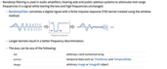
- バンドパスフィルタリングは,音声増幅器,補聴器,拡声装置にしばしば使われるもので,信号の高周波数および低周波数はそのまま残しつつ中間波数を減衰させる.
- BandstopFilterは,窓法で作成された有限インパルス応答 (FIR) カーネルを使用してデジタル信号をたたみ込みむ
- カーネルが長くなると周波数の識別が向上する.
- data は次のいずれでもよい.
-
list 任意階数の数値配列 tseries TimeSeriesやTemporalDataのような時間データ image 任意のImageオブジェクトまたはImage3Dオブジェクト audio AudioオブジェクトまたはSoundオブジェクト video Videoオブジェクト - 減衰される周波数の範囲はカットオフ周波数 ω1および ω2 (ω2>ω1)に依存する.
- 画像や多次元配列に適用された場合,フィルタリングはレベル1から始めて各次元に連続的に適用される.BandstopFilter[data,{{ω11,ω21},…}]は i 次元で周波数{ω1i,ω2i}を使う.
- 周波数値 ωiは0から
まででなければならない. - BandstopFilter[data,{ω1,ω2}]はカットオフ周波数{ω1,ω2}と入力 data に適したフィルタカーネル長と平滑化窓を使う.
- よく使われる平滑化窓 wfun
-
BlackmanWindow Blackman窓で平滑化する DirichletWindow 平滑化は行わない HammingWindow ハミング窓で平滑化する {v1,v2,…} 値 viの窓を使う f
から
の範囲で f をサンプリングすることで窓を作る - 使用可能なオプション
-
Padding "Fixed" 使用する充填値 SampleRate Automatic 入力に想定されるサンプルレート - デフォルトで,データと同様画像にもSampleRate->1が想定される.音声信号と時系列については,サンプルレートは抽出されるか入力データから計算されるかする.
- SampleRatesr の場合,カットオフ周波数 ωcは0から sr
まででなければならない.
例題
すべて開く すべて閉じる例 (3)
data = Table[Cos[x] + Cos[10x] + Cos[20x], {x, 0, 2Pi, 0.04}];
filtered = BandstopFilter[data, {.2, .6}, 31];
ListLinePlot[{data, filtered}, PlotLegends -> {"original", "filtered"}]ideal = Table[Cos[x] + Cos[20x], {x, 0, 2Pi, 0.04}];
ListLinePlot[{ideal, filtered}]BandstopFilter[\!\(\*AudioBox[""]\), {Quantity[500, "Hertz"], Quantity[2500, "Hertz"]}]BandstopFilter[[image], {0.25, 1.}]//ImageAdjustスコープ (13)
データ (8)
data = BoxMatrix[5, {41}];
ListLinePlot[{data, BandstopFilter[data, {.5, 1.5}, 15]}, PlotRange -> All]data = Table[UnitBox[(n/7), (m/7)], {n, -7, 7}, {m, -7, 7}];
ListPlot3D[data]BandstopFilter[data, {0.5, 1.5}]//ListPlot3DTimeSeriesにフィルタをかける:
ts = TemporalData[TimeSeries, {{{0., -0.27267267057145633, -0.6672983789995302, -0.5338541947930846,
-0.6117404489279314, -0.6755527076595494, -0.02125421294486496, -0.10792797291843935,
-0.6138271235477938, -0.3248568606554575, -0.08843449054 ... 2053424, -0.49980440691873723, -0.5388679788215971,
-0.4101602764645551}}, {{0, 1., 0.01}}, 1, {"Continuous", 1}, {"Continuous", 1}, 1,
{ValueDimensions -> 1, ResamplingMethod -> {"Interpolation", InterpolationOrder -> 1}}}, False,
10.1];
filtered = BandstopFilter[ts, {Quantity[5, "Hertz"], Quantity[10, "Hertz"]}];ListLinePlot[{ts, filtered}, PlotLegends -> {"original data", "filtered"}]3全音信号のSoundオブジェクトにバンドストップフィルタをかける:
snd = Sound[SampledSoundList[Table[Sin[2 π 697 t] + Sin[2 π 1209 t] + Sin[2π 1633 t], {t, 0., 0.3, 1 / 8000.}], 8000]]長さ101のBlackman窓でバンドストップフィルタを使って中間の音を除去する:
BandstopFilter[snd, {Quantity[900, "Hertz"], Quantity[1400, "Hertz"]}, 101, BlackmanWindow]BandstopFilter[[image], {0.5, 1.}]BandstopFilter[Video["ExampleData/fish.mp4"], {0.5, 1}]BandstopFilter[[image], {0.5, 1.}]BandstopFilter[{0, 0, 0, 1, 1, 1, 0, 0, 0}, {Pi / 2, Pi}, 5]パラメータ (5)
数値カットオフ周波数は弧度秒を単位とした数量として解釈される:
a = \!\(\*AudioBox[""]\);BandstopFilter[a, {2000 π, 4000 π}] === BandstopFilter[a, {Quantity[2000*Pi, "Radians"/"Seconds"], Quantity[4000*Pi, "Radians"/"Seconds"]}] === BandstopFilter[a, {Quantity[1000, "Hertz"], Quantity[2000, "Hertz"]}]カットオフ周波数が
と
のバンドストップフィルタを使ってホワイトノイズ信号にフィルタをかける:
noise = AudioGenerator["White", 0.2];
Periodogram[noise]Periodogram[BandstopFilter[noise, {Quantity[5000, "Hertz"], Quantity[15000, "Hertz"]}]]Periodogram[BandstopFilter[noise, {{Quantity[8660, "Hertz"], 1}}]]Periodogram[BandstopFilter[noise, {{Quantity[8660, "Hertz"], 0.66}}]]noise = AudioGenerator["White", 0.2];
Periodogram[BandstopFilter[noise, {Quantity[5000, "Hertz"], Quantity[15000, "Hertz"]}, 33]]Periodogram[BandstopFilter[noise, {Quantity[5000, "Hertz"], Quantity[15000, "Hertz"]}, 55]]a = AudioGenerator[Sin[11025 2 π #^2]&];
Periodogram[BandstopFilter[a, {Quantity[5000, "Hertz"], Quantity[15000, "Hertz"]}, 33, #]& /@ {DirichletWindow, HammingWindow, BlackmanWindow}, PlotLegends -> {"Dirichlet", "Hamming", "Hann"}]調節可能なカイザー(Kaiser)窓を使って減衰量を変える:
Periodogram[Table[BandstopFilter[a, {Quantity[5000, "Hertz"], Quantity[15000, "Hertz"]}, 33, KaiserWindow[#, b]&], {b, {3, 5, 7}}], PlotLegends -> {3, 5, 7}]BandstopFilter[[image], {{0.5, 1.33}, {0.75, 1.}}, 33]オプション (3)
Padding (1)
SampleRate (2)
サンプルレート sr=1を仮定して周波数 π/2に中心を置くフィルタを使う:
BandstopFilter[{0, 0, 0, 0, 0, 1, 1, 1, 1, 1}, {{π / 2., 1}}]BandstopFilter[{0, 0, 0, 0, 0, 1, 1, 1, 1, 1}, {{3π / 2., 1}}, SampleRate -> 3]レート
でサンプリングされた音声にバンドストップフィルタを適用する:
noise = AudioGenerator["White", 0.2];
sr = QuantityMagnitude@AudioSampleRate[noise]BandstopFilter[noise, {{sr π / 2., 1}}]//Periodogramアプリケーション (1)
現代の88鍵のピアノでは,55番目のキー(C5)の基本周波数は約523Hzである.BandstopFilterを使って,以下の音声クリップにあるその他の周波数は保持しつつ,このキーの最初の倍音(1046Hz) を効率的に削除する:
key55 = \!\(\*AudioBox[""]\);基本周波数(1046Hz)を中心とした長さ101の狭いフィルタ(Q=3)を使う:
f = 2 523;
res = BandstopFilter[key55, {{2 π f, 3}}, 101]Periodogram[{key55, res}, PlotRange -> All, GridLines -> All, PlotLegends -> {"original", "filtered"}]特性と関係 (5)
BandstopFilter[{0., 0., 0., 0., 1., 1., 1., 1.}, {0, Pi}]LeastSquaresFilterKernelおよびハミング窓を使ってバンドストップフィルタを作る:
n = 5;
ω = {1, 1.5};
win = Array[HammingWindow, n, {-1 / 2, 1 / 2}];
ker = win LeastSquaresFilterKernel[{"Bandstop", ω}, n]ListConvolve[ker, {0, 0, 0, 1, 1, 1, 0, 0, 0}, Ceiling[n / 2], 0]BandstopFilterの結果と比較する:
BandstopFilter[{0, 0, 0, 1, 1, 1, 0, 0, 0}, ω, n, win, Padding -> 0]h = BandstopFilter[ArrayPad[{1}, 10], {0.5, 2.5}, 21]ListPlot[h, PlotRange -> All, Filling -> 0]Plot[Abs[ListFourierSequenceTransform[h, ω]], {ω, 0, π}]平滑化窓なしでの長さ21のバンドストップフィルタのインパルス応答:
h = BandstopFilter[ArrayPad[{1}, 10], {0.5, 2.5}, 21, None]ListPlot[h, PlotRange -> All, Filling -> 0]Plot[Abs[ListFourierSequenceTransform[h, ω]], {ω, 0, π}]バンドストップフィルタの周波数弁別はフィルタの長さが長くなるにつれて向上する:
Manipulate[
ListLinePlot[Abs[Fourier[BandstopFilter[ArrayPad[{1.}, 128], {Pi / 4., 3 Pi / 4.}, n, None], FourierParameters -> {1, -1}]][[ ;; 129]], ...], {{n, 21}, 3, 63, 2}]関連するガイド
テキスト
Wolfram Research (2012), BandstopFilter, Wolfram言語関数, https://reference.wolfram.com/language/ref/BandstopFilter.html (2025年に更新).
CMS
Wolfram Language. 2012. "BandstopFilter." Wolfram Language & System Documentation Center. Wolfram Research. Last Modified 2025. https://reference.wolfram.com/language/ref/BandstopFilter.html.
APA
Wolfram Language. (2012). BandstopFilter. Wolfram Language & System Documentation Center. Retrieved from https://reference.wolfram.com/language/ref/BandstopFilter.html
BibTeX
@misc{reference.wolfram_2026_bandstopfilter, author="Wolfram Research", title="{BandstopFilter}", year="2025", howpublished="\url{https://reference.wolfram.com/language/ref/BandstopFilter.html}", note=[Accessed: 08-September-2026]}
BibLaTeX
@online{reference.wolfram_2026_bandstopfilter, organization={Wolfram Research}, title={BandstopFilter}, year={2025}, url={https://reference.wolfram.com/language/ref/BandstopFilter.html}, note=[Accessed: 08-September-2026]}