ConvexOptimization[f,cons,vars]
求可最小化受凸约束条件 cons 限制的凸目标函数 f 的变量 vars 的值.
ConvexOptimization[…,"prop"]
指定应返回解的属性 "prop".
ConvexOptimization
ConvexOptimization[f,cons,vars]
求可最小化受凸约束条件 cons 限制的凸目标函数 f 的变量 vars 的值.
ConvexOptimization[…,"prop"]
指定应返回解的属性 "prop".
更多信息和选项
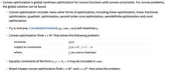
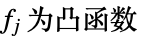
- 凸优化是受凸约束条件限制的凸函数的全局非线性最优化. 对于凸问题,可以找到全局解.
- 凸优化包括许多其他形式的优化,包括线性优化、线性分数优化、二次优化、二阶锥优化、半正定优化和锥优化等.
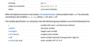
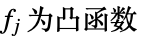
- 如果
是凹函数,则 ConvexOptimization[-g,cons,vars] 将使 g 最大化. - 凸优化求的是可解下列问题的
: -
最小化 
受限于约束条件 
其中 
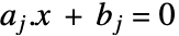
- 可将形为
的等式约束条件包括在 cons 中. - 混合整数凸优化求的是
和
,以求解下列问题: -
最小化 
受限于约束条件 
其中 
- 当目标函数为实值时,ConvexOptimization 通过内部转换为实数变量
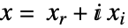
来求解
,其中
和
. - 变量指定 vars 应该是一个列表,其中包含以下列形式之一给出变量的元素:
-
v 名为
和推断尺寸的变量v∈Reals 实数标量变量 v∈Integers 整数标量变量 v∈Complexes 复数标量变量 v∈ℛ 限制在几何区域
的向量变量v∈Vectors[n,dom] 属于
、
或
的向量变量v∈Matrices[{m,n},dom] 属于
、
或
的矩阵变量 - ConvexOptimization 自动进行必要的转换,以找到解决最小化问题的有效方法.
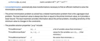
- 所求解的原始最小化问题有一个相关的最大化问题,即拉格朗日对偶问题. 对偶最大值始终小于或等于原始最小值,因此它提供了一个下限. 对偶最大化程序提供有关原始问题的信息,包括最小值对约束变化的敏感性.
- 可能的解的属性 "prop" 包括:
-
"PrimalMinimizer" 
最小化
的变量值列表"PrimalMinimizerRules" 
最小化
的变量值 vars={v1,…}"PrimalMinimizerVector" 
最小化
的向量"PrimalMinimumValue" 
最小值
"DualMaximizer" 
最大化对偶问题的向量 "DualMaximumValue" 对偶最大值 "DualityGap" 
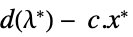
对偶最优值和原最优值之差 "Slack" 
将不等式约束转换为等式的向量 "ConstraintSensitivity"
对约束摄动的敏感性{"prop1","prop2",…} 解的多个属性 - 可以给出以下选项:
-
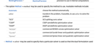
MaxIterations Automatic 使用的最大迭代次数 Method Automatic 使用方法 PerformanceGoal $PerformanceGoal 优化的目标 Tolerance Automatic 内部比较使用的公差 WorkingPrecision MachinePrecision 内部计算使用的精度 - 选项 Methodmethod 可以用来指定要使用的方法. 可用的方法包括:
-
Automatic 自动选择方法 solver 可能的情况下,对问题进行转换,用 solver 求解问题 "SCS" SCS 劈分圆锥求解器 "CSDP" CSDP 半定优化求解器 "DSDP" DSDP 半定优化求解器 "MOSEK" 商用 MOSEK 凸优化求解器 "Gurobi" 商用 Gurobi 线性和二次优化求解器 "Xpress" 商用 Xpress 线性和二次优化求解器 - Methodsolver 可以用来指定使用特定的求解器,以使所用的对偶公式对应于为 solver 所收录的公式. 可能的求解器有 LinearOptimization、LinearFractionalOptimization、QuadraticOptimization、 SecondOrderConeOptimization、SemidefiniteOptimization、ConicOptimization 和 GeometricOptimization.
范例
打开所有单元 关闭所有单元基本范例 (2)
ConvexOptimization[Abs[x + 2 y], {x + y == 1., x - y ≤ 2}, {x, y}]ConvexOptimization[Norm[x], {Indexed[x, {1, 2}] == 1, Indexed[x, {2, 3}] == 2, Indexed[x, {1, 1}] ≤ Indexed[3x, {2, 1}] + Indexed[2x, {1, 3}], Indexed[x, {2, 2}] == Indexed[x, {1, 1}] + 7}, {x∈Matrices[{2, 3}, Reals]}]范围 (28)
基本用法 (12)
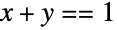
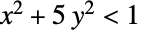
ConvexOptimization[x^2 + y^2, {x + y == 1, x ^ 2 + 5y ^ 2 < 1}, {x, y}]几个线性不等式约束可以使用 VectorGreaterEqual 表示:
ConvexOptimization[x + y, VectorGreaterEqual[{{x + 2y, x}, {3, -1}}], {x, y}]使用
v>=
或者 \[VectorGreaterEqual] 输入向量不等式符号 :
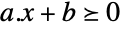
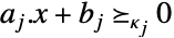
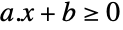
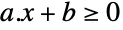
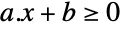
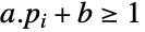
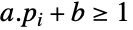
ConvexOptimization[x + y, {x + 2y, x}{3, -1}, {x, y}]ConvexOptimization[x + y, {x + 2y ≥ 3, x ≥ -1}, {x, y}]ConvexOptimization[{1, 1}.v, {{1, 2}, {1, 0}}.v{3, -1}, v]ConvexOptimization[{1, 1}.x, {{1, 2}, {1, 0}}.x + {-3, 1}0, x]ConvexOptimization[{1, 1}.x, {{1, 2}, {1, 0}}.x{3, -1}, x]要避免在
中的意外线程,使用 Inactive[Plus]:
ConvexOptimization[{1, 1}.x, {{1, 2}, {1, 0}}.x + {-3, 1}0, x]parEqs = {a == {{1, 2}, {1, 0}}, b == {3, -1}};ConvexOptimization[{1, 1}.x, {parEqs, a.x + b0}, x]VectorGreaterEqual 表示关于 "NonNegativeCone" 的圆锥不等式:
constraint = VectorGreaterEqual[{{{1, 2}, {1, 0}}.v, {3, -1}}, "NonNegativeCone"]明确指定圆锥的尺寸,使用 {"NonNegativeCone",n}:
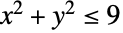
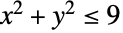
constraint = VectorGreaterEqual[{{{1, 2}, {1, 0}}.v, {3, -1}}, {"NonNegativeCone", 2}]ConvexOptimization[{1, 1}.v, constraint, v]ConvexOptimization[x + 2y, x^2 + y^2 ≤ 9, {x, y}]VectorGreaterEqual[{{x, y, 3}, 0}, {"NormCone", 3}]ConvexOptimization[x + 2y, {x, y, 3}Underscript[, {"NormCone", 3}]0, {x, y}]constraint = VectorGreaterEqual[{{{x, 1}, {1, y}}, 0}, {"SemidefiniteCone", 2}]ConvexOptimization[x + 2y, constraint, {x, y}]使用向量变量
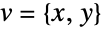
和 Indexed[x,i] 以指定单个分量:
ConvexOptimization[{1, 2}.x, (| | |
| --------------- | --------------- |
| Indexed[x, {1}] | 1 |
| 1 | Indexed[x, {2}] |)Underscript[, {"SemidefiniteCone", 2}]0, x]使用 Vectors[n,Reals] 在向量变量可能不明确时指定其尺寸:
ConvexOptimization[Indexed[x, {1}] + 2Indexed[x, {2}], (| | |
| --------------- | --------------- |
| Indexed[x, {1}] | 1 |
| 1 | Indexed[x, {2}] |)Underscript[, {"SemidefiniteCone", 2}]0, x]ConvexOptimization[Indexed[x, {1}] + Indexed[2x, {2}], (| | |
| --------------- | --------------- |
| Indexed[x, {1}] | 1 |
| 1 | Indexed[x, {2}] |)Underscript[, {"SemidefiniteCone", 2}]0, x∈Vectors[2, Reals]]使用 NonNegativeReals (
) 指定非负约束:
ConvexOptimization[{-1, -2}.x, Norm[x] ≤ 1, x∈Vectors[2, NonNegativeReals]]ConvexOptimization[{-1, -2}.x, {Norm[x] ≤ 1, x0}, x]ConvexOptimization[(1/w h), {2w + 2h ≤ 1, h ≤ (1/2)w}, {h, w}]当
和
为正时,该问题可以通过 GeometricOptimization 方法求解:
ConvexOptimization[(1/w h), {2w + 2h ≤ 1, h ≤ (1/2)w, h ≥ 0, w ≥ 0}, {h, w}]使用方法 GeometricOptimization 隐式假定为正:
ConvexOptimization[(1/w h), {2w + 2h ≤ 1, h ≤ (1/2)w}, {h, w}, Method -> GeometricOptimization]整数变量 (4)
使用 Integers 指定整数变量:
ConvexOptimization[x ^ 2 + y ^ 2, {x + 2y ≥ 2}, {x∈Integers, y∈Integers}]使用 Vectors[n,Integers] 指定向量变量的整数域约束:
ConvexOptimization[Total[x], {a == {{1, 2}, {1, 0}}, b == {3, -2},
a.xb}, {x∈Vectors[2, Integers]}]使用 NonNegativeIntegers (
)指定非负整数域约束:
ConvexOptimization[x + 2y, {x^2 + 2y^2 ≤ 3, x + y == 2, x∈NonNegativeIntegers}, {x, y}]使用 NonPositiveIntegers (
)指定非正整数域约束:
ConvexOptimization[-x + y, {x + 2y ≥ 3, x∈NonPositiveIntegers}, {x, y}]复数变量 (8)
使用 Complexes 指定复变量:
ConvexOptimization[Re[z] + Im[z], Abs[z] ≤ 2, z∈ Complexes]constraints = VectorGreaterEqual[{(-1 + 2I) z, -3}] && VectorGreaterEqual[{z, I}]VectorGreaterEqual /@ ComplexExpand[constraints[[All, 1]] /. z -> x + I y]realConstraints = -x - 2y ≥ -3 && 2 x - y ≥ 0 && x ≥ 0 && y ≥ 1;RegionPlot[realConstraints, {x, 0.5, 1}, {y, 1, 1.2}]ConvexOptimization[Re[z], constraints, Element[z, Complexes]]ConvexOptimization[x, realConstraints, {x, y}]{q, c} = {{{2, 1 + I}, {1 - I, 1}}, {2, 3}};
ConvexOptimization[(1 / 2) * x.q.x + c.x, {}, x∈Vectors[2, Reals]]使用含有埃尔米特矩阵
和复变量的目标函数 (1/2)Inactive[Dot][Conjugate[x],q,x]:
q = {{1, I}, {-I, 2}};
ConvexOptimization[(1 / 2) * Inactive[Dot][Conjugate[x], q, x] , {{1, I}.x1 + I}, x∈Vectors[2, Complexes]]{q, c} = {{{2, 1 + I}, {1 - I, 1}}, {2, 3}};
ConvexOptimization[{1, 2}.x, (1 / 2) * x.q.x + c.x1, x∈Vectors[2, Reals]]使用含有埃尔米特矩阵
和复变量的约束条件 (1/2)Inactive[Dot][Conjugate[x],q,x]d:
q = {{3, 1 + I}, {1 - I, 2}};
ConvexOptimization[{1, 2}.Re[x], {(1 / 2) * Inactive[Dot][Conjugate[x], q, x]5}, x∈Vectors[2, Complexes]]求具有最小2-范数(最大奇异值)的埃尔米特矩阵,使得矩阵
为半正定:
ConvexOptimization[Norm[x], VectorGreaterEqual[{x, {{1, I}, {-I, 1}}}, "SemidefiniteCone"], Element[x, Matrices[{2, 2}, Complexes, Hermitian]]]Norm[x] /. %Subscript[a, 0] = (| | |
| ----- | ----- |
| 0 | 1 + I |
| 1 - I | 0 |);Subscript[a, 1] = (| | |
| - | - |
| 1 | 0 |
| 0 | 0 |);Subscript[a, 2] = (| | |
| - | - |
| 0 | 0 |
| 0 | 1 |);线性矩阵不等式中的变量必须是实数才能使和保持为埃尔米特矩阵:
c = {1, 2};
ConvexOptimization[c.v, {Subscript[a, 1], Subscript[a, 2]}.vUnderscript[, {"SemidefiniteCone", 2}]-Subscript[a, 0], v∈Vectors[2, Reals]]原模型属性 (1)
triangle = {x ≥ 0, y ≥ 0, x + 2y ≤ 2};
disk = x ^ 2 + y ^ 2 ≤ 1;sol = ConvexOptimization[-(x + y), {triangle, disk}, {x, y}]{xmin, ymin} = ConvexOptimization[-(x + y), {triangle, disk}, {x, y}, "PrimalMinimizer"]minval = ConvexOptimization[-(x + y), {triangle, disk}, {x, y}, "PrimalMinimumValue"]RegionPlot[{x ≥ 0 && y ≥ 0 && x + 2 y ≤ 2, x ^ 2 + y ^ 2 ≤ 1}, {x, 0, 2}, {y, 0, 1}, AspectRatio -> Automatic, Epilog -> {Red, PointSize[0.025], Point[{x, y} /. sol]}]对偶模型属性 (3)
c = {1, 1};
Subscript[a, 0] = {{1., -1.}}; Subscript[b, 0] = {0};
Subscript[a, 1] = {{1., 0}, {0, 1}, {0, 0}};Subscript[b, 1] = {0, 0, 1};psol = ConvexOptimization[c.x, {Subscript[a, 0].x + Subscript[b, 0] == 0, Subscript[a, 1].x + Subscript[b, 1]Underscript[, {"NormCone", 3}]0}, x]dsol = ConvexOptimization[Subscript[b, 0].Subscript[λ, 0] + Subscript[b, 1].Subscript[λ, 1] , {Transpose[Subscript[a, 0]].Subscript[λ, 0] + Transpose[Subscript[a, 1]].Subscript[λ, 1] == c, Subscript[λ, 1]Underscript[, {"NormCone", 3}]0}, {Subscript[λ, 0], Subscript[λ, 1]}]{c.x /. psol, -Subscript[b, 0].Subscript[λ, 0] - Subscript[b, 1].Subscript[λ, 1] /. dsol}ConvexOptimization[c.x, {Subscript[a, 0].x + Subscript[b, 0] == 0, Subscript[a, 1].x + Subscript[b, 1]Underscript[, {"NormCone", 3}]0}, x, "DualityGap"]c = {1, 1};
Subscript[a, 0] = {{1., -1.}}; Subscript[b, 0] = {0};
Subscript[a, 1] = {{1., 0}, {0, 1}, {0, 0}};Subscript[b, 1] = {0, 0, 1};ConvexOptimization[c.x, {Subscript[a, 0].x + Subscript[b, 0] == 0, Subscript[a, 1].x + Subscript[b, 1]Underscript[, {"NormCone", 3}]0}, x, "DualMaximumValue"]ConicOptimization[Indexed[x, {1}] + Indexed[x, {2}], {Indexed[x, {1}] == Indexed[x, {2}], Indexed[x, {1}]^2 + Indexed[x, {2}]^2 ≤ 1}, {Indexed[x, {1}], Indexed[x, {2}]}, "DualMaximumValue"]dualMaximizer = ConicOptimization[Indexed[x, {1}] + Indexed[x, {2}], {Indexed[x, {1}] == Indexed[x, {2}], Indexed[x, {1}]^2 + Indexed[x, {2}]^2 ≤ 1}, {Indexed[x, {1}], Indexed[x, {2}]}, "DualMaximizer"]{Subscript[λ, 0], Subscript[λ, 1]} = dualMaximizer要获取特定问题类型求解程序的对偶格式,需将其指定为方法选项:
ConvexOptimization[x - y, {x ≥ 0, y ≥ 0, x + 2 y ≤ 3}, {x, y}, "DualMaximizer", Method -> LinearOptimization]LinearOptimization[x - y, {x ≥ 0, y ≥ 0, x + 2 y ≤ 3}, {x, y}, "DualMaximizer"]选项 (13)
Method (8)
ConvexOptimization[-x - y, {x ≥ 0, y ≥ 0, x + 2y ≤ 2, x^2 + y^2 ≤ 1}, {x, y}, Method -> "SCS"]ConvexOptimization[-x - y, {x ≥ 0, y ≥ 0, x + 2y ≤ 2, x^2 + y^2 ≤ 1}, {x, y}, Method -> "CSDP"]ConvexOptimization[-x - y, {x ≥ 0, y ≥ 0, x + 2y ≤ 2, x^2 + y^2 ≤ 1}, {x, y}, Method -> "DSDP"]ConvexOptimization[-x - y, {x ≥ 0, y ≥ 0, x + 2y ≤ 2, x^2 + y^2 ≤ 1}, {x, y}, Method -> "IPOPT"]{obj, cons, var} = {-x - y, {x ≥ 0, y ≥ 0, x + 2y ≤ 2, x ^ 2 + y ^ 2 ≤ 1}, {x, y}};
props = {"PrimalMinimumValue", "PrimalMinimizer"};{minval, argmin} = Minimize[obj, cons, var];
exact = {minval, var /. argmin};solSCS = ConvexOptimization[obj, cons, var, props, Method -> "SCS"];solCSDP = ConvexOptimization[obj, cons, var, props, Method -> "CSDP"];solDSDP = ConvexOptimization[obj, cons, var, props, Method -> "DSDP"];solIPOPT = ConvexOptimization[obj, cons, var, props, Method -> "IPOPT"];solSCS - exact"CSDP"、"DSDP" 和 "IPOPT" 的默认公差为
:
solCSDP - exactsolDSDP - exactsolIPOPT - exact当指定方法 "SCS" 时,将调用该方法并使用 SCS 库的默认公差 10-3:
ConvexOptimization[x + y, {x^2 + y^2 ≤ 1}, {x, y}, Method -> "SCS"]当使用默认选项时,该问题可通过公差为 10-6 的方法 "SCS" 求解:
ConvexOptimization[x + y, {x^2 + y^2 ≤ 1}, {x, y}]ConvexOptimization[x + y, {x^2 + y^2 ≤ 1}, {x, y}, Method -> {"SCS", Tolerance -> 10 ^ -6}]对转换为半定约束的约束使用方法 "CSDP" 或 "DSDP":
lin = {{1, 0}, {0, 1}, {-1, -2}}.x + {0, 0, 2}Underscript[, {"NonNegativeCone", 3}]0;norm = {{1, 0}, {0, 1}, {0, 0}}.x + {0, 0, 1}Underscript[, {"NormCone", 3}]0;semi = {{{-4, 0}, {0, 0}}, {{0, 0}, {0, -0.8}}}.x + {{5, 1}, {1, 1}}Underscript[, {"SemidefiniteCone", 2}]0;ConvexOptimization[{-1, -1}.x, {lin, norm, semi}, x, Method -> "CSDP"]ConvexOptimization[{-1, -1}.x, {lin, norm, semi}, x, Method -> "DSDP"]当 "CSDP" 和 "DSDP" 不适用时,使用方法 "IPOPT" 获取精确解:
expConstraint = {{1, 0}, {0, 1}, {-1, -2}}.x + {0, 0, 2}Underscript[, "ExponentialCone"]0;powConstraint = {{1, 0}, {0, 1}, {-1, -2}}.x + {1, 0, 2}Underscript[, {"PowerCone", (1/3)}]0;"IPOPT" 生成比 "SCS" 更准确的结果,但通常要慢得多:
AbsoluteTiming[xmin = ConvexOptimization[{1, 1}.x, {expConstraint, powConstraint}, x, Method -> "IPOPT"]]AbsoluteTiming[xmin = ConvexOptimization[{1, 1}.x, {expConstraint, powConstraint}, x, Method -> "SCS"]]PerformanceGoal (1)
选项 PerformanceGoal 的默认值为 $PerformanceGoal:
$PerformanceGoal使用 PerformanceGoal"Quality" 以获得更准确的结果:
ConvexOptimization[x + y, {Norm[{x, y}] ≤ Sqrt[2], {x, y}1}, {x, y},
"PrimalMinimumValue", PerformanceGoal -> "Quality"]ConvexOptimization[x + y, {Norm[{x, y}] ≤ Sqrt[2], {x, y}1}, {x, y},
"PrimalMinimumValue", PerformanceGoal -> "Speed"]使用 PerformanceGoal"Speed" 可以更快地获得结果,但以牺牲质量为代价:
n = 100000; {obj, const, vars} = {Total[x] / n, {Norm[x] ≤ Sqrt[n], x1}, x∈Vectors[n]};Timing[resSpeed = ConvexOptimization[obj, const, vars,
"PrimalMinimumValue", PerformanceGoal -> "Speed"];]Timing[resQuality = ConvexOptimization[obj, const, vars,
"PrimalMinimumValue", PerformanceGoal -> "Quality"];]{resSpeed, resQuality}Tolerance (2)
较小的 Tolerance 设置给出更精确的结果:
{obj, cons, var} = {-x - y, {x ≥ 0, y ≥ 0, x + 2y ≤ 2, x ^ 2 + y ^ 2 ≤ 1}, {x, y}};使用 Minimize 计算确切的最小值:
exact = Minimize[obj, cons, var][[1]]用不同的 Tolerance 设置计算最小值的误差:
err = Table[{tol, Abs[ConvexOptimization[obj, cons, var, "PrimalMinimumValue", Tolerance -> tol] - exact]}, {tol, 10. ^ -Range[7]}]ListLogLogPlot[err, PlotRange -> All, Joined -> True, PlotMarkers -> Automatic]较小的 Tolerance 设置会给出更精确的答案,但计算需要的时间可能更长:
n = 100000; {obj, const, vars} = {Total[x] / n, {Norm[x] ≤ Sqrt[n], x1}, x∈Vectors[n]};Timing[ptight = ConvexOptimization[obj, const, vars,
"PrimalMinimumValue", Tolerance -> 10^-12];]Timing[ploose = ConvexOptimization[obj, const, vars,
"PrimalMinimumValue", Tolerance -> 10^-2];]{ptight, ploose}WorkingPrecision (2)
默认工作精度为 MachinePrecision:
ConvexOptimization[x - y, {x ≥ 2, y ≥ 0, x + 2 y ≤ 3}, {x, y}]如果可能,使用 WorkingPrecisionInfinity 将给出确切的解:
ConvexOptimization[x - y, {x ≥ 2, y ≥ 0, x + 2 y ≤ 3}, {x, y}, WorkingPrecision -> ∞]WorkingPrecision 而不是 MachinePrecision 和 ∞ 将尝试使用具有扩展精度支持的方法:
ConvexOptimization[x - y, {x ≥ 2, y ≥ 0, x + 2 y ≤ 3}, {x, y}, WorkingPrecision -> 20]使用 WorkingPrecisionAutomatic 将尝试使用输入问题的精度:
ConvexOptimization[x - y, {x ≥ 2, y ≥ 0, x + 2 y ≤ 3}, {x, y}, WorkingPrecision -> Automatic]ConvexOptimization[x - y, {x ≥ 2.0, y ≥ 0.0, x + 2 y ≤ 3.0}, {x, y}, WorkingPrecision -> Automatic]ConvexOptimization[(x - y) ^ 2, {x ≥ 2, y ≥ 0, x + 2 y ≤ 3}, {x, y}, WorkingPrecision -> 20]当前没有使用精确算法求解二次目标问题的方法. 当不支持所要求的精度时,则计算使用机器数:

ConvexOptimization[(x - y) ^ 2, {x ≥ 2, y ≥ 0, x + 2 y ≤ 3}, {x, y}, WorkingPrecision -> ∞]应用 (30)
基本模型变换 (11)
最大化约束为
的
. 通过对目标函数进行负转换来求解最大化问题:
ConvexOptimization[-(x + y), {x + y == 3, x ≥ 0, y ≤ 2}, {x, y}]-ConvexOptimization[-(x + y), {x + y == 3, x ≥ 0, y ≤ 2}, {x, y}, "PrimalMinimumValue"]最小化约束为
的
. 由于约束
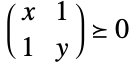
非凸,因此使用半定约束使凸性明确:
constraint = VectorGreaterEqual[{{{x, 1}, {1, y}}, 0}, "SemidefiniteCone"]当且仅当矩阵的所有左上子矩阵的行列式均为非负值时,才是正半定矩阵:
{Det[{{x}}] ≥ 0, Det[{{x, 1}, {1, y}}] ≥ 0}ConvexOptimization[2 x + 3 y, constraint, {x, y}]最小化
,约束为
,假定当
时,
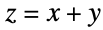
成立. 使用辅助变量
,目标变为最小化
,使得
:
{α, β, γ, δ} = {{1, 2}, 1, {-3, 4}, 2};
{a, b} = {{{1, -2}, {-3, 4}}, {-5, -1}};Reduce[Implies[a.{Indexed[x, {1}], Indexed[x, {2}]} + b >= 0, γ.{Indexed[x, {1}], Indexed[x, {2}]} + δ > 0], Reals]舒尔补条件是指,如果
,当且仅当
时,分块矩阵
. 因此当且仅当
时,
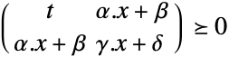
. 使用 Inactive[Plus] 构造约束以避免线程化:
ConvexOptimization[t, {(| | |
| ------- | ------- |
| t | α.x + β |
| α.x + β | γ.x + δ |)Underscript[, {"SemidefiniteCone", 2}]0, a.x + b0}, {t, x∈Vectors[2]}]ConvexOptimization[Norm[x], {x∈Disk[{1, 1}, {2, 1}]}, {x}]上镜图(Epigraph)变换可用于构造具有线性目标以及附加变量和约束的问题:
ConvexOptimization[t, {Norm[x] ≤ t, x∈Disk[{1, 1}, {2, 1}]}, {x, t}]这种形式的问题可以直接使用 ConicOptimization 求解:
ConicOptimization[t, {Norm[x] ≤ t, x∈Disk[{1, 1}, {2, 1}]}, {x, t}]通过最小化
来最小化
,其中
是非递减函数. 对于这两个问题,原始最小化器
将保持不变. 考虑最小化
,其约束为
:
f = Function[{s}, Sqrt[s]];{minval, Subscript[z, min]} = ConvexOptimization[x + y, {(| | |
| - | - |
| x | 1 |
| 1 | y |)Underscript[, {"SemidefiniteCone", 2}]0, x + y ≥ 0}, {x, y}, {"PrimalMinimumValue", "PrimalMinimizerRules"}]f[minval]ConvexOptimization 将自动执行此转换:
ConvexOptimization[f[x + y], {(| | |
| - | - |
| x | 1 |
| 1 | y |)Underscript[, {"SemidefiniteCone", 2}]0, x + y ≥ 0}, {x, y}, {"PrimalMinimumValue", "PrimalMinimizerRules"}]求
,使得线性依赖于决策变量
的对称矩阵
的最大特征值最小. 由于
等价于
,其中
是
的第 ![]()
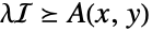
个特征值,该问题可以表述为线性矩阵不等式. 定义线性矩阵函数
:
A[x_, y_] := (| | |
| -- | -- |
| 2 | -3 |
| -3 | 4 |) + (| | |
| - | - |
| 1 | 2 |
| 2 | 3 |) x + (| | |
| - | - |
| 4 | 5 |
| 5 | 6 |) yA[x, y]//MatrixForm实对称矩阵
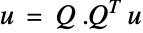
可以用正交矩阵
对角线化使得
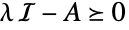
. 因此当且仅当
时,
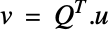
. 由于任何
,认为
,
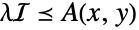
,因此当且仅当
时,
. 数值模拟表明这些公式是等效的:
eigs = Eigenvalues[A[1., 2.]]data = Table[{λ, λ (| | |
| - | - |
| 1 | 0 |
| 0 | 1 |) Underscript[, {"SemidefiniteCone", 2}]A[1., 2.]}, {λ, RandomReal[{0, 35}, 100]}];
{true, false} = {Cases[data, {λ_, True} :> λ], Cases[data, {λ_, False} :> λ]};NumberLinePlot[{eigs, true, false}, IconizedObject[«Rule»]]res = ConvexOptimization[λ, λ (| | |
| - | - |
| 1 | 0 |
| 0 | 1 |) Underscript[, {"SemidefiniteCone", 2}]A[x, y], {λ, x, y}]Min[Table[Max[Eigenvalues[A@@RandomReal[{-10000, 10000}, 2]]], 10000]]求
,使的对称于决策变量
的对称矩阵
的最小特征值最大. 定义线性矩阵函数
:
A[x_, y_] := (| | |
| ------------- | ------------- |
| x + 4 y + 2 | 2 x + 5 y - 3 |
| 2 x + 5 y - 3 | 3 x + 6 y + 4 |);这个问题可以表述为线性矩阵不等式,因为
等价于
,其中
是
的第
个特征值. 要最大化
,需最小化
:
res = ConvexOptimization[-λ,
λ (| | |
| - | - |
| 1 | 0 |
| 0 | 1 |) Underscript[, {"SemidefiniteCone", 2}]A[x, y], {λ, x, y}]Max[Table[Min[Eigenvalues[A@@RandomReal[{-10000, 10000}, 2]]], 10000]]求
,使得线性依赖于决策变量
的对称矩阵
的最大和最小特征值之差最小. 定义线性矩阵函数
:
A[x_, y_] := (| | |
| ------------- | ------------- |
| x + 4 y + 2 | 2 x + 5 y - 3 |
| 2 x + 5 y - 3 | 3 x + 6 y + 4 |);这个问题可以表述为线性矩阵不等式,由于
等价于
,其中
是
的第
个特征值. 求解得到的问题:
res = ConvexOptimization[μ - λ, {λ (| | |
| - | - |
| 1 | 0 |
| 0 | 1 |) Underscript[, {"SemidefiniteCone", 2}]A[x, y]Underscript[, {"SemidefiniteCone", 2}]μ (| | |
| - | - |
| 1 | 0 |
| 0 | 1 |)}, {λ, μ, x, y}]{Eigenvalues[A[x, y] /. res], Chop[μ - λ /. res, 10 ^ -7]}最小化线性依赖于决策变量
的对称矩阵
的最大特征值(按绝对值):
A[x_, y_] := (| | |
| ------------- | ------------- |
| x + 4 y + 2 | 2 x + 5 y - 3 |
| 2 x + 5 y - 3 | 3 x + 6 y + 4 |);最大特征值满足
的最大(按绝对值)负特征值是
的最大特征值并满足
:
res = ConvexOptimization[λ, {-λ (| | |
| - | - |
| 1 | 0 |
| 0 | 1 |)Underscript[, {"SemidefiniteCone", 2}]A[x, y]Underscript[, {"SemidefiniteCone", 2}]λ (| | |
| - | - |
| 1 | 0 |
| 0 | 1 |)}, {λ, x, y}]Eigenvalues[A[x, y] /. res]求
,使得线性依赖于决策变量
的对称矩阵
的最大奇异值
最小化:
A[x_, y_] := (| | | |
| ----------- | ----------- | ----- |
| 1 + x + 2 y | 2 + 3 y | x + 1 |
| 3 + 5 y | 4 - x + 8 y | 2y |);
的最大奇异值
是
的最大特征值的平方根,并且根据前面的示例,它满足
,或者等价于
:
res = ConvexOptimization[σ, **{****{****σ** (| | |
| - | - |
| 1 | 0 |
| 0 | 1 |)**, ****A[x, y]****}****, ****{****A[x, y]****, ****σ** (| | | |
| - | - | - |
| 1 | 0 | 0 |
| 0 | 1 | 0 |
| 0 | 0 | 1 |)**}****}** Underscript[, {"SemidefiniteCone", 5}]0, {x, y, **σ**}]f[x_, y_] := Module[{v = SingularValueList[A[x, y]]}, Max[v]];
Show[Plot3D[f[x, y], {x, -10, 10}, {y, -2, 2}], Graphics3D[{Red, PointSize[.05], Point[res[[All, 2]]]}]]对于包括椭圆体、二次锥和抛物面在内的二次集合
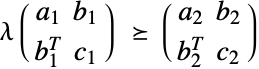
,确定
是否成立,其中
是对称矩阵,
为向量,
为标量:
{a1, b1, c1} = {{{0.7, 0.68}, {0.68, 0.94}}, {0.35, .42}, 0.12};{a2, b2, c2} = {{{0.13, 0.2}, {0.2, 0.62}}, {.2, .4}, .01};With[{x = {x1, x2}}, RegionPlot[{x.a1.x + 2 b1.x + c1 ≤ 0, x.a2.x + 2 b2.x + c2 ≤ 0}, {x1, -2, 2}, {x2, -2, 2}, PlotLegends -> {Subscript[𝒬, 1], Subscript[𝒬, 2]}, ImageSize -> 100]]假定集合
是全维度的,S-procedure 表示,当且仅当存在某个非负数
使得
成立时,
. 直观地看到存在一个非负数
:
m1 = ArrayFlatten[{{a1, {b1}}, {{b1}, {{c1}}}}];
m2 = ArrayFlatten[{{a2, {b2}}, {{b2}, {{c2}}}}];
Plot[Boole[λm1Underscript[, {"SemidefiniteCone", 3}]m2], {λ, 0, 5}, ImageSize -> Small]考虑到可行性,将 0 用作目标函数. 由于 λ≥0,因此
:
ConvexOptimization[0, λ(| | |
| -- | -- |
| a1 | b1 |
| b1 | c1 |)Underscript[, {"SemidefiniteCone", 3}](| | |
| -- | -- |
| a2 | b2 |
| b2 | c2 |), λ]几何问题 (8)
最小化面积为 4 的矩形的对角线长度,使得宽度加上高度的三倍小于 7:
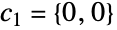
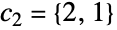
ConvexOptimization[Sqrt[w ^ 2 + h ^ 2], {w h == 4, w + 3h ≤ 7, h ≥ 0, w ≥ 0}, {w, h}]求半径为 1 的两个圆盘之间的最小距离,圆盘的中心分别为
和
. 设
为圆盘 1 上的一个点. 设
为 圆盘 2 上的一个点. 目标是最小化
,约束为
:
res = ConvexOptimization[Norm[p1 - p2], {c2 == {2, 1}, Norm[p1] ≤ 1, Norm[p2 - c2] ≤ 1}, {p1∈Vectors[2], p2∈Vectors[2]}]Graphics[{{Lighter[Blue], Disk[]}, {Lighter[Red], Disk[{2, 1}]}, {Green, PointSize[0.03], Point[{p1, p2} /. res]}}]EuclideanDistance[p1, p2] /. resvolume = (4/3)π a b c;surfaceArea = 4π ((a^pb^p + a^pc^p + b^p c^p/3))^1 / p /. p -> 1.6075;ConvexOptimization[1 / volume, {surfaceArea ≤ 1, a ≥ 0, b ≥ 0, c ≥ 0}, {a, b, c}]结果是一个球. 如果对轴的长度附加约束条件将使结果发生改变:
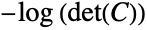
ConvexOptimization[1 / volume, {surfaceArea ≤ 1, 3b + a ≤ 1, a ≥ 0, b ≥ 0, c ≥ 0}, {a, b, c}]Graphics3D[Ellipsoid[{0, 0, 0}, {a, b, c} /. %]]region = [image];constraints = Table[Norm[Inactive[Plus][pi, -c]] ≤ r, {pi, MeshCoordinates[region]}];res = ConvexOptimization[r, constraints, {r, c∈Vectors[3]}]Show[Graphics3D[{Opacity[0.2], Red, Ball[c, r] /. res}], region]可通过 BoundingRegion 高效地找到最小包含球:
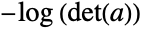
BoundingRegion[region, "MinBall"]求凸多边形的解析中心. 解析中心是使约束的距离乘积最大化的点:
cmesh = ConvexHullMesh[IconizedObject[«With»]];凸多边形的每个边可以表示为半平面
的交线. 提取线性不等式:
{a, b} = LinearOptimization[0, x∈cmesh, x, "LinearInequalityConstraints"];objective = Total[Table[-Log[a[[i]].x + b[[i]]], {i, Length[a]}]];res = ConvexOptimization[objective, {}, {x}, Method -> {"SCS", Tolerance -> 10 ^ -7}]Show[cmesh, Graphics[{PointSize[0.02], Point[x /. res]}]]{a1, b1, c1} = {{{0.13, 0.2}, {0.2, 0.62}}, {.2, .4}, .01};
{a2, b2, c2} = {{{0.7, 0.68}, {0.68, 0.94}}, {0.35, .42}, 0.12};使用 S-procedure 可以证明,当且仅当
时,椭圆 2 是椭圆 1 的子集:
subsetConstraint = (| | |
| -- | -- |
| a1 | b1 |
| b1 | c1 |)Underscript[, {"SemidefiniteCone", 3}]τ(| | |
| -- | -- |
| a2 | b2 |
| b2 | c2 |);ConvexOptimization[0, {subsetConstraint, τ ≥ 0}, τ]ellipse1 = With[{ai = Inverse[a1]}, Ellipsoid[-ai.b1, ai(b1.ai.b1 - c1)]];
ellipse2 = With[{ai = Inverse[a2]}, Ellipsoid[-ai.b2, ai(b2.ai.b2 - c2)]];Graphics[{{Red, Opacity[0.5], ellipse1}, {Blue, Opacity[0.5], ellipse2}}]{a3, b3, c3} = {{{0.7, 0.68}, {0.68, 0.94}}, {0.45, .42}, 0.12};
ellipse3 = With[{ai = Inverse[a3]}, Ellipsoid[-ai.b3, ai(b3.ai.b3 - c3)]];现在进行测试表明该问题是不可行的,这表明椭球 2 不是椭球 1 的子集:
ConvexOptimization[0, {(| | |
| -- | -- |
| a1 | b1 |
| b1 | c1 |)Underscript[, {"SemidefiniteCone", 3}]τ(| | |
| -- | -- |
| a3 | b3 |
| b3 | c3 |), τ ≥ 0}, τ];Graphics[{{Red, Opacity[0.5], ellipse1}, {Blue, Opacity[0.5], ellipse3}}]cmesh = ConvexHullMesh[IconizedObject[«With»]];segs = MeshPrimitives[cmesh, 1][[All, 1]];
a = segs /. {p_, q_} :> {-1, 1} * Reverse[p - q];
b = MapThread[#1.#2&, {a, segs[[All, 1]]}];将参数化应用于半平面,可以得出
. 项
. 因此,约束条件为
:
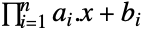
constraints = Table[Norm[a[[i]].c] + a[[i]].d ≤ b[[i]], {i, Length[a]}];res = ConvexOptimization[-Tr[c], constraints, {c∈Matrices[{2, 2}], d}]inscribedEllipse = Ellipsoid[d, Transpose[c].c] /. resShow[cmesh, Graphics[{Purple, inscribedEllipse}]]通过最小化体积,找到参数化为
、包括三维中的一组点的最小椭球体:
pts = IconizedObject[«With»];constraints = Table[Norm[a.pi + b] ≤ 1, {pi, pts}];res = ConvexOptimization[-Tr[a], {constraints, aUnderscript[, {"SemidefiniteCone", 3}]0}, {a, b∈Vectors[3]}]{Σ, x0} = {Inverse[Transpose[a].a /. res], -LinearSolve[a, b] /. res};
minVolEllipsoid = Ellipsoid[x0, Σ]Graphics3D[{{Opacity[0.3], Red, Ellipsoid[x0, Σ]}, {PointSize[0.025], Point[pts]}}]也可以使用 BoundingRegion 得到包围椭圆体(体积不一定是最小的):
fastEllipsoid = BoundingRegion[pts, "FastEllipsoid"]{Volume[minVolEllipsoid], Volume[fastEllipsoid]}数据拟合问题 (4)
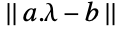
{a, b} = IconizedObject[«Block»];ConvexOptimization[Norm[Inactive[Plus][a.x, -b]], x1, {x}]将三次曲线拟合到离散数据,以使数据的第一个和最后一个点位于曲线上:
data = IconizedObject[«Block»];使用 DesignMatrix 构造矩阵:
a = DesignMatrix[data, {1, x, x^2, x^3}, x];
b = data[[All, 2]];pointConstraints = {a[[1]].λ == b[[1]], a[[-1]].λ == b[[-1]]};res = ConvexOptimization[Norm[Inactive[Plus][a.λ, -b]], pointConstraints, {λ}]Show[Plot[Evaluate[{1, x, x^2, x^3}.λ /. res], {x, 0, 1}, Epilog -> {Red, PointSize[0.03], Point[data[[{1, -1}]]]}], ListPlot[data]]data = IconizedObject[«Block»];bases = Sqrt[1 + (x - #) ^ 2]& /@ Subdivide[-3, 3, 10];
input = DesignMatrix[data, bases, x, IncludeConstantBasis -> False];
output = data[[All, 2]];res = ConvexOptimization[Norm[Inactive[Plus][a.λ, -b], 1], {a == input, b == output}, {λ}]Plot[Evaluate[bases.λ /. res], {x, -3, 3}, Epilog -> {PointSize[0.008], Point[data]}]Plot[{Sin[2x] + Cos[x ^ 2], Evaluate[bases.λ /. res]}, {x, -3, 3}, PlotLegends -> {"Reference", "SubscriptBox[L, 1]fit"}]data = Block[{z}, SeedRandom[1234];
Table[{z = RandomComplex[{-2 - 2I, 2 + 2I}], z ^ (3 / 2) + 0.02 RandomComplex[]}, {i, 100}]];对于基
,使用 DesignMatrix 构建矩阵
:
basis = {1, z, z ^ 2, z ^ 3};
a = DesignMatrix[data, basis, z];
b = data[[All, 2]];With[{σ = 0.2, m = Length[basis]}, res = ConvexOptimization[Norm[Inactive[Plus][a.λ, -b]] + σ Norm[λ, 1], {}, {Element[λ, Vectors[m, Complexes]]}]]f[x_, y_] := basis.λ /. res /. z -> x + I y;Show[Plot3D[Re[f[x, y]], {x, -2, 2}, {y, -2, 2}], Graphics3D[{PointSize[0.03], Blue, Point[MapThread[Append, {ReIm[data[[All, 1]]], Re[data[[All, 2]]]}]]}]]Show[Plot3D[Im[f[x, y]], {x, -2, 2}, {y, -2, 2}], Graphics3D[{PointSize[0.03], Red, Point[MapThread[Append, {ReIm[data[[All, 1]]], Im[data[[All, 2]]]}]]}]]平方和表示 (1)
poly = 2 + 4 x + 6 x^2 + 4 x^3 + x^4;v = {1, x, x^2};n = Length[v];
mat = Array[Indexed[q, {##}] &, {n, n}];
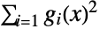
Q = UpperTriangularize[mat] + Transpose[UpperTriangularize[mat, 1]];coeffs = Map[# == 0&, DeleteCases[Flatten[CoefficientList[v.Q.v - poly, {x}]], 0]]res = ConvexOptimization[0, {coeffs , qUnderscript[, {"SemidefiniteCone", n}]0}, q]二次项
,其中
是由
的 Cholesky 分解获得的下三角矩阵:
L = CholeskyDecomposition[(Q /. res)];
g = L.v;
Expand[Sum[g[[i]]^2, {i, Length[g]}]]Chop[Expand[Total[g ^ 2]] - poly, 10^-7]分类问题 (3)
{set1, set2} = IconizedObject[«Block»];constraints = {set1.a + b1, set2.a + b-1};res = ConvexOptimization[Norm[a], constraints, {a, b}]line = a.{x, y} + b /. resShow[RegionPlot[line ≤ 0, {x, 0, 1}, {y, 0, 1}], ListPlot[{set1, set2}, PlotMarkers -> {Automatic, PointSize[0.025]}]]{set1, set2} = IconizedObject[«Block»];
dataplot = ListPointPlot3D[{set1, set2}, Sequence[...]]使用 DesignMatrix 构造两个集合的二次多项式数据矩阵:
{data1, data2} = DesignMatrix[#, {x, x^2, y, y^2, x y}, {x, y}]& /@ {set1, set2};constraints = {data1.a + b1, data2.a + b-1};res = ConvexOptimization[Norm[a], constraints, {a, b}, Tolerance -> 10 ^ -3]poly = (a.{1, x, x^2, y, y^2, x y} + b) /. resShow[dataplot, ContourPlot3D[poly == 0, {x, -1.5, 1.5}, {y, -1.5, 1.5}, {z, -1, 1}, Sequence[...]]]将给定的点集
分成不同的组. 这通过最小化
以找到每个组的中心
得到,其中
是给定的本地内核,
是给定的惩罚参数:
x = IconizedObject[«Block»];
{n, dim} = Dimensions[x];
centers = Indexed[μ, #]& /@ Range[n];内核
是
-近邻(
)函数,使得
,或者
. 对于此问题,选择
个最近邻:
kNN = Nearest[x -> Automatic][x, 10];
κ = SparseArray[Join@@Table[Thread[{i, kNN[[i]]}], {i, n}] -> 1, {n, n}];c1 = Table[Norm[Inactive[Plus][Indexed[x, {i}], -Indexed[μ, {i}]]], {i, n}];
c2 = Flatten[Table[κ[[i, j]]Norm[Indexed[μ, {i}] - Indexed[μ, {j}], 1], {i, 1, n}, {j, i + 1, n}]];
objective = Total[c1 ^ 2] / 2 + 10 Total[c2];vars = Table[Indexed[μ, {i}]∈Vectors[dim, Reals], {i, n}];res = ConvexOptimization[objective, {}, vars];对于每个数据点,都有一个对应的中心. 属于同一组的数据将具有相同的中心值:
allCenters = centers /. res;
cvals = Map[First, Gather[allCenters, Norm[#1 - #2] ≤ 0.001&]]gpts = Table[Pick[x, Map[Norm[# - ci] ≤ 0.001&, allCenters]], {ci, cvals}];
Show[ListPlot[gpts, PlotStyle -> PointSize[0.02]], ListPlot[allCenters, PlotStyle -> {PointSize[0.03], Yellow}]]设施选址问题 (1)
clientPos = {{0, 0}, {1, 0}, {3 / 2, 1}, {-1 / 2, 1}, {1 / 2, 3 / 2}, {1 / 2, 1 / 2}, {0, 3 / 2}, {1, 1}, {0, 1}, {3 / 2, 3 / 2}};
nTowers = 3;
nClients = Length[clientPos];每个基站消耗的功率与其范围成正比,由
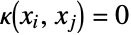
给出. 目的是最大程度地降低功耗:
objective = Sum[r[i] ^ 1.5, {i, nTowers}];decisionConstraint = 0z1;m = 20;
distConstraint = Table[Norm[Inactive[Plus][p[j], -clientPos[[i]]]] -
m * (1 - Indexed[z, {i, j}]) ≤ r[j], {i, nClients}, {j, nTowers}];coverageConstraint = Total[z, {2}]1;maxCoverageConstraint = Table[0 ≤ r[j] ≤ 1, {j, nTowers}];vars = Flatten[{Table[{p[j]∈Vectors[2], r[j]}, {j, nTowers}], z∈Matrices[{nClients, nTowers}, Integers]}];res = Quiet[ConvexOptimization[objective, {decisionConstraint,
distConstraint, coverageConstraint, maxCoverageConstraint}, vars]]towerPos = Table[p[i], {i, nTowers}] /. res;
towerRange = Table[r[i], {i, nTowers}] /. res;Graphics[{{Orange, PointSize[0.04], Point[towerPos]}, {Blue, PointSize[0.02], Point[clientPos]}, {...}}, Frame -> True]投资组合优化 (1)
求如何在六只股票之间分配资本
,在最大程度地降低风险的同时最大化回报:
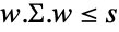
{μ, Σ} = Block[...];return = μ.w;risk = w.Σ.w;
riskConstraint = risk ≤ s;目标是最大化收益,同时在指定的风险规避参数的情况下最大程度地降低风险:
objective[α_ ? NumericQ] := -(return - α s);可用
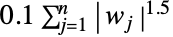
模拟买卖股票对股票市场价格的影响,该模型通过上镜图变换用幂锥来模拟:
marketConstraints = Table[Abs[Indexed[w, i]] ^ 1.5 ≤ Indexed[t, i], {i, 6}];weightConstraints = {w0, Total[w] + 0.1Total[t] == 1};frontier = Table[res = Quiet@ConvexOptimization[objective[α],
{riskConstraint, weightConstraints, marketConstraints}, {w, s, t∈Vectors[6]}];
{risk, return} /. res, {α, Subdivide[0, 10, 200]}];randomRiskReturns = Table[{risk, return}, {w, Table[...]}];
Show[ListPlot[frontier, ...], ListPlot[randomRiskReturns, Rule[...]]]riskAversionParameter = N@{1 / 1000, 1 / 100, 1 / 2, 1, 5, 10, 15, 20};
res = Table[{α, return, Quiet@Append[w, 1 - Total[w]]} /.
Quiet@ConicOptimization[objective[α],
{riskConstraint, weightConstraints, marketConstraints}, {w, s, t∈Vectors[6]}], {α, riskAversionParameter}];通过考虑市场成本,可以获得低风险规避参数的多样化投资组合,但是当风险规避参数较高时,由于购买的是分散程度较低的股票,市场影响成本占主导地位:
BarChart[res[[All, -1]], ChartLayout -> "Stacked", ChartLabels -> {riskAversionParameter, None}, Axes -> False, Frame -> True, ChartLegends -> SwatchLegend[Automatic, Append[(StringForm["Stock ``", #]&) /@ Range[6], "market impact cost"], LegendLabel -> "Stock"], FrameLabel -> {"Risk Aversion Parameter", "Fraction of budget"}]图像处理 (1)
image = ImageResize[ColorConvert[ExampleData[{"TestImage", "House"}], "Grayscale"], 75]data = ImageData[image];
SeedRandom[123];
mask = RandomChoice[{0.4, 0.6} -> {0, 1}, Dimensions[data]];
corruptedData = mask * data;
Image[corruptedData]{n, m} = Dimensions[data];objective = Total[Flatten[Table[Norm[{Indexed[u, {i + 1, j}] - Indexed[u, {i, j}], Indexed[u, {i, j + 1}] - Indexed[u, {i, j}]}], {i, n - 1}, {j, m - 1}]]];knownPos = SparseArray[mask]["NonzeroPositions"];constraint = Map[Indexed[u, #] == data[[Sequence@@#]]&, knownPos];sol = ConvexOptimization[objective, constraint, u∈Matrices[{n, m}]];Image[u /. sol]相关指南
-
▪
- 凸优化 ▪
- 最优化 ▪
- 符号向量、矩阵和数组
文本
Wolfram Research (2020),ConvexOptimization,Wolfram 语言函数,https://reference.wolfram.com/language/ref/ConvexOptimization.html.
CMS
Wolfram 语言. 2020. "ConvexOptimization." Wolfram 语言与系统参考资料中心. Wolfram Research. https://reference.wolfram.com/language/ref/ConvexOptimization.html.
APA
Wolfram 语言. (2020). ConvexOptimization. Wolfram 语言与系统参考资料中心. 追溯自 https://reference.wolfram.com/language/ref/ConvexOptimization.html 年
BibTeX
@misc{reference.wolfram_2026_convexoptimization, author="Wolfram Research", title="{ConvexOptimization}", year="2020", howpublished="\url{https://reference.wolfram.com/language/ref/ConvexOptimization.html}", note=[Accessed: 16-September-2026]}
BibLaTeX
@online{reference.wolfram_2026_convexoptimization, organization={Wolfram Research}, title={ConvexOptimization}, year={2020}, url={https://reference.wolfram.com/language/ref/ConvexOptimization.html}, note=[Accessed: 16-September-2026]}