Wolfram言語＆システムドキュメントセンター

CorrelationFunction

CorrelationFunction[data,hspec]

data からの遅れ hspec における相関関数を推定する．

CorrelationFunction[proc,hspec]

遅れ hspec におけるランダム過程 proc の相関関数を表す．

CorrelationFunction[proc,s,t]

時間 s および t におけるランダム過程 proc の相関関数を表す．

詳細

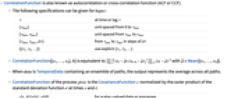
CorrelationFunctionは自己相関関数(ACF)あるいは相互相関関数(CCF)としても知られている．
hspec には次の指定を使うことができる．

	τ	時間または遅れ τ で
	{τ_max}	0から τ_maxまで等間隔で
	{τ_min,τ_max}	τ_minから τ_maxまで等間隔で
	{τ_min,τ_max,dτ}	τ_min から τ_maxまで刻み幅 dτ で
	{{τ₁,τ₂,…}}	明示的な{τ₁,τ₂,…}を使う

CorrelationFunction[{x₁,…,x_n},h]は =Mean[{x₁,…,x_n}]であるに等しい．
data が，経路の集合体を含むTemporalDataであるとき，その出力はすべての経路の平均を表す．
過程 proc のCorrelationFunctionは，時間 s および t における，標準偏差関数 σ の外積によって正規化されたCovarianceFunction c である．

	c[s,t]/(σ[s]σ[t])	スカラー値のデータまたは過程について
	c[s,t]/(σ[s] ⊗ σ[t])	ベクトル値のデータまたは過程について

記号 ⊗ はKroneckerProductである．
CorrelationFunction[proc,h]は proc が弱定常過程でCorrelationFunction[proc,h,0]と等しいときにのみ定義される．
過程 proc はARMAProcessまたはWienerProcessのような任意のランダム過程である．

例題

すべて開くすべて閉じる

例 (4)

遅れ2での相関関数を推定する：

Wolfram Language code: CorrelationFunction[{2, 3, 4, 3}, 2]

自己回帰時系列からのランダムサンプルのサンプル相関関数：

Wolfram Language code: data = RandomFunction[ARProcess[{.2, .3, .4}, 1], {1, 10 ^ 4}];

Wolfram Language code: ListPlot[CorrelationFunction[data, {20}], Filling -> Axis, PlotRange -> All]

離散時間過程の相関関数：

Wolfram Language code: CorrelationFunction[BinomialProcess[p], s, t]

Wolfram Language code: DiscretePlot3D[Evaluate[% /. {p -> 2 / 3}], {s, 1, 10}, {t, 1, 10}, ExtentSize -> 1 / 2, ColorFunction -> "Rainbow"]

連続時間過程の相関関数：

Wolfram Language code: CorrelationFunction[WienerProcess[μ, σ], s, t]

Wolfram Language code: Plot3D[Evaluate[% /. {μ -> 1, σ -> 2}], {s, 0, 10}, {t, 0, 10}, ColorFunction -> "Rainbow"]

スコープ (13)

経験的推定値 (7)

遅れ9におけるデータについて相関関数を推定する：

Wolfram Language code: CorrelationFunction[Range[10], 9]

遅れ9までの相関関数の経験的推定値を得る：

Wolfram Language code: CorrelationFunction[Range[10], {9}]

刻み幅2で遅れ1から9までの相関関数を計算する：

Wolfram Language code: CorrelationFunction[Range[10], {1, 9, 2}]

時系列についての相関関数を計算する：

Wolfram Language code:

ts = TemporalData[TimeSeries, {{{-2.9904395734335427, -1.5547517217370468, -2.007044987914736, 
    -0.7114933373063236, -1.5920036118254968, 0.23183536513859127, 0.056774681349179124, 
    0.32394041932443046, 0.10382798659711348, -0.684046765274114, - ... 1687325555, 
    3.410933732368106, 2.5200924558212163, 2.008558601261935, 0.43151331467691206, 
    0.6249727955196763}}, {{1, 1000, 1}}, 1, {"Continuous", 1}, {"Discrete", 1}, 1, 
  {ValueDimensions -> 1, ResamplingMethod -> None}}, False, 10.1];

複数の遅れについての時系列の相関関数は，時系列として返される：

Wolfram Language code: corr = CorrelationFunction[ts, {100}]

Wolfram Language code: ListPlot[corr, Filling -> Axis]

経路の集合体について相関関数を推定する：

Wolfram Language code: data = RandomFunction[ARProcess[{.8}, 1], {0, 500}, 10]

Wolfram Language code: corr = CorrelationFunction[data, {12}];

Wolfram Language code: ListPlot[corr, Filling -> 0]

経験的な相関関数と理論上の相関関数を比べる：

Wolfram Language code: proc = MAProcess[{.4, .3, .5, .6, .3}, 1.];

Wolfram Language code: data = RandomFunction[proc, {0, 1000}];

Wolfram Language code:

ListPlot[TemporalData[CorrelationFunction[#, {10}]& /@ {proc, data}], Filling -> {1 -> {2}}, PlotStyle -> PointSize[Medium]]

ベクトルデータについて，相互相関をプロットする：

Wolfram Language code:

proc = ARProcess[{{{.3, .1}, {.6, .3}}}, {{1, .3}, {.3, .6}}];
data = RandomFunction[proc, {100}];
cov = CorrelationFunction[data, {-6, 6}];

Wolfram Language code: Table[ListPlot[cov["Values"][[All, i, j]], Filling -> 0, PlotLabel -> {i, j}], {i, 1, 2}, {j, 1, 2}]

ランダム過程 (6)

弱定常離散時間過程の相関関数：

Wolfram Language code: CorrelationFunction[ARProcess[{a}, σ^2], s, t]//PiecewiseExpand

Wolfram Language code:

DiscretePlot3D[Evaluate[% /. {a -> 2 / 3, σ -> 1}], {s, 0, 10}, {t, 0, 10}, ExtentSize -> 1 / 2, ColorFunction -> "Rainbow"]

相関関数は反対角のみに依存する：

Wolfram Language code: CorrelationFunction[ARProcess[{a}, σ^2], h]//PiecewiseExpand

Wolfram Language code:

DiscretePlot[Evaluate[% /. {a -> 2 / 3, σ -> 1}], {h, 0, 10}, ExtentSize -> 1 / 2, ColorFunction -> "Rainbow", AxesLabel -> {h, None}]

弱定常連続時間過程の相関関数：

Wolfram Language code: CorrelationFunction[OrnsteinUhlenbeckProcess[μ, σ, θ], s, t]

Wolfram Language code: Plot3D[Evaluate[% /. {μ -> 1, σ -> 2, θ -> 1 / 3}], {s, 0, 10}, {t, 0, 10}, ColorFunction -> "Rainbow"]

相関関数は反対角のみに依存する：

Wolfram Language code: CorrelationFunction[OrnsteinUhlenbeckProcess[μ, σ, θ], h]

Wolfram Language code:

Plot[Evaluate[% /. {μ -> 1, σ -> 2, θ -> 1 / 3}], {h, 0, 10}, ColorFunction -> "Rainbow", Filling -> Axis, AxesLabel -> {h, None}]

弱定常ではない離散時間過程の相関関数：

Wolfram Language code: CorrelationFunction[BinomialProcess[p], s, t]

Wolfram Language code: DiscretePlot3D[Evaluate[% /. p -> 1 / 3], {s, 1, 10}, {t, 1, 10}, ExtentSize -> 1 / 2, ColorFunction -> "Rainbow"]

相関関数は，両方の時間引数に依存する：

Wolfram Language code: antidiagonals = CorrelationFunction[BinomialProcess[1 / 3], t, t + h]

Wolfram Language code:

DiscretePlot[Evaluate@Table[antidiagonals, {t, 1, 4}], {h, 0, 5}, ExtentSize -> 1 / 2, PlotLegends -> (Row[{"t = ", #}]& /@ Range[1, 4]), AxesLabel -> {h, None}]

弱定常ではない連続時間過程の相関関数：

Wolfram Language code: CorrelationFunction[PoissonProcess[μ], s, t]

Wolfram Language code: Plot3D[Evaluate[% /. μ -> 3], {s, 0, 10}, {t, 0, 10}, ColorFunction -> "Rainbow"]

相関関数は，両方の時間引数に依存する：

Wolfram Language code: antidiagonals = CorrelationFunction[PoissonProcess[3], t, t + h]

Wolfram Language code:

Plot[Evaluate@Table[antidiagonals, {t, 1, 4}], {h, 0, 5}, PlotLegends -> (Row[{"t = ", #}]& /@ Range[1, 4]), AxesLabel -> {h, None}]

いくつかの時系列過程の相関関数：

Wolfram Language code:

proc1 = ARProcess[{.8}, 1];
proc2 = MAProcess[{-.4, -.7, .6, -1}, 1];
proc3 = SARMAProcess[{}, {}, {3, {.6}, {.1}}, 1];
proc4 = FARIMAProcess[{}, 1 / 3, {}, 1];

Wolfram Language code:

DiscretePlot[CorrelationFunction[#, h], {h, 0, 15}, ExtentSize -> 1 / 2, PlotRange -> All, PlotLabel -> Head[#]]& /@ {proc1, proc2, proc3, proc4}

ベクトルARProcessについての相互相関プロット：

Wolfram Language code:

proc = ARProcess[{{{.3, .1}, {.6, .3}}}, {{1, .3}, {.3, .6}}];
cov = CorrelationFunction[proc, h];

Wolfram Language code: Table[DiscretePlot[cov[[i, j]], {h, -6, 6}, ExtentSize -> 1 / 2, PlotLabel -> {i, j}], {i, 1, 2}, {j, 1, 2}]

アプリケーション (2)

次のデータはMAProcessあるいはARProcessのどちらを使った場合に最もよくモデル化ができるかを考える：

Wolfram Language code:

ListLinePlot[data = TemporalData[TimeSeries, {{{-1.4735257611469446, -0.9158187257309729, -1.9060205147226934, 
    -1.6174582169404574, -2.633459084244463, -2.104839842098871, -2.8701276893108894, 
    -2.4118183939601607, -0.5125633448622677, -1.2356329399850385, 1. ... 26394036266876, -0.16380797769527589, 0.3559909972777121, 
    1.5343047104249412, 0.10763337590714506}}, {{0, 100, 1}}, 1, {"Continuous", 1}, 
  {"Discrete", 1}, 1, {ResamplingMethod -> {"Interpolation", InterpolationOrder -> 1}}}, False, 
 10.1]]

もとになっている過程をサンプル経路から決定するのは難しい：

Wolfram Language code: candidates = {MAProcess[{.5, .4}, 1], ARProcess[{.5, .4}, 1]};

Wolfram Language code: SeedRandom[2];ListLinePlot[RandomFunction[#, {0, 100}]]& /@ candidates

データの相関関数は徐々に減衰する：

Wolfram Language code: ListPlot[CorrelationFunction[data, {10}], Filling -> 0]

ARProcessは明らかにMAProcessよりもよいモデル候補である：

Wolfram Language code: ListPlot[CorrelationFunction[#, {10}], PlotLabel -> Head[#], Filling -> 0]& /@ candidates

ホワイトノイズの信頼帯を含む自己相関関数(ACF)プロットを作成する：

Wolfram Language code: data = RandomFunction[MAProcess[{.6, .4, .5}, .1], {1, 500}];

Wolfram Language code:

acf[data_, lmax_, clev_ : 0.95] := Show[ListPlot[CorrelationFunction[data, {0, lmax}], Filling -> Axis, PlotRange -> {{0, lmax}, All}, PlotStyle -> PointSize[Medium]], 
	Graphics[{Dashed, Line[{{0, #}, {lmax, #}}]}]& /@ (Quantile[NormalDistribution[], {(1 - clev/2), 1 - (1 - clev/2)}]/Sqrt[data["PathLengths"][[1]]])]

95%のホワイトノイズ信頼帯で遅れ0から20までについて相関をプロットする：

Wolfram Language code: acf[data, 20, .95]

非相関のホワイトノイズと比べる：

Wolfram Language code: acf[TemporalData[RandomVariate[NormalDistribution[], 500], Automatic], 20, .95]

特性と関係 (12)

サンプル相関関数は，過程の相関関数のバイアス推定器である：

Wolfram Language code:

proc = ARMAProcess[1, {5 / 6, -1 / 6}, {2 / 3}, 1];
paths = RandomFunction[proc, {0, n = 10}, 10 ^ 3];

サンプル相関関数を計算する：

Wolfram Language code: CorrelationFunction[paths, {10}]

Wolfram Language code: scorr = TimeSeriesMapThread[#2(n + 1) / (n + 1 - #1)&, %]

この過程についての相関関数：

Wolfram Language code: corr = CorrelationFunction[proc, {10}]

両関数をプロットする：

Wolfram Language code: ListPlot[{scorr, corr}, Filling -> 0]

過程についての相関関数は，Correlation行列の非対角項である：

Wolfram Language code: 𝒫 = WienerProcess[μ, σ];

Wolfram Language code: Correlation[𝒫[{s, t}], 1, 2]

Wolfram Language code: CorrelationFunction[𝒫, s, t]

Wolfram Language code: Simplify[%% - %, 0 < s < t]

遅れ0におけるサンプル相関は常に1である：

Wolfram Language code: Simplify[CorrelationFunction[{x, y, z}, 0], {x, y, z}∈Reals]

サンプル相関関数は，CovarianceFunctionに関連している：

Wolfram Language code: data = Range[10];

Wolfram Language code: CorrelationFunction[data, {Length[data] - 1}]

スケールされたサンプル共分散関数：

Wolfram Language code: CovarianceFunction[data, {Length[data] - 1}] / CovarianceFunction[data, 0]

Wolfram Language code: % - %%

サンプル相関関数は，AbsoluteCorrelationFunctionに関連している：

Wolfram Language code:

data = Range[10];
n = Length[data];

Wolfram Language code: AbsoluteCorrelationFunction[data - Mean[data], {n - 1}]

第1要素でスケールする：

Wolfram Language code: % / First[%]

サンプル相関関数と比べる：

Wolfram Language code: CorrelationFunction[data, {n - 1}]

Wolfram Language code: % - %%

Expectationを使って相関を計算する：

Wolfram Language code: 𝒫 = WienerProcess[μ, σ];

平均と標準偏差の関数を定義する：

Wolfram Language code:

sd[s_] := StandardDeviation[𝒫[s]]
m[s_] := Mean[𝒫[s]]

Wolfram Language code: Expectation[(x[s] - m[s])(x[t] - m[t]) / (sd[s] sd[t]), x𝒫]

Wolfram Language code: CorrelationFunction[𝒫, s, t]

Wolfram Language code: Simplify[% - %%, 0 < s < t]

等しい時間に対する相関関数は1に簡約される：

Wolfram Language code: CorrelationFunction[PoissonProcess[μ], t, t]//Simplify[#, t > 0]&

相関関数は，CovarianceFunction に関連している：

Wolfram Language code:

𝒫 = OrnsteinUhlenbeckProcess[μ, σ, θ];
sd[s_] := StandardDeviation[𝒫[s]]

Wolfram Language code: CorrelationFunction[𝒫, s, t]

については，標準偏差関数はである：

Wolfram Language code: CovarianceFunction[𝒫, s, t] / (sd[s] sd[t])

Wolfram Language code: % - %%

相関関数は，Correlationに関連している：

Wolfram Language code: 𝒫 = WienerProcess[μ, σ];

Wolfram Language code: CorrelationFunction[𝒫, s, t]

これは，共分散行列における非対角項である：

Wolfram Language code: Correlation[𝒫[{s, t}], 1, 2]

Wolfram Language code: Simplify[%% - %, 0 < s < t]

相関関数は，ToInvertibleTimeSeriesについては不変である：

Wolfram Language code: TimeSeriesInvertibility[proc = MAProcess[{2, 4}, 1]]

Wolfram Language code: iproc = ToInvertibleTimeSeries@proc

Wolfram Language code: CorrelationFunction[#, s, t]& /@ {proc, iproc}

相関関数は，中心化しても変わらない：

Wolfram Language code: data = RandomFunction[ARIMAProcess[{}, 1, {}, 1], {0, 100}];

データは非零の平均を持つ：

Wolfram Language code: Mean[data]

データを中心に集める：

Wolfram Language code: newdata = Standardize[data, Mean, 1&];

相関関数を比べる：

Wolfram Language code: ListPlot[CorrelationFunction[#, {20}], Filling -> 0]& /@ {data, newdata}

サンプル相関関数の和は一定である：

Wolfram Language code:

n = 100;
sample = RandomInteger[n, n];

サンプルはランダムである：

Wolfram Language code: ListPlot[sample, Filling -> Axis]

1からn-1までのサンプル相関関数を計算する：

Wolfram Language code:

corr = CorrelationFunction[sample, {1, n - 1}];
ListLinePlot[corr]

和を計算する：

Wolfram Language code: Total@corr

考えられる問題 (1)

CorrelationFunctionの出力がDifferenceRootを含むことがある：

Wolfram Language code: CorrelationFunction[ARProcess[{a, b}, σ^2], t] //Simplify[#, t > 0]&

FunctionExpandを使って明示的なベキを回復する：

Wolfram Language code: %//FunctionExpand

Top

その他のラーニングリソース

テクニカルサポート

データサイエンス，金融，ビジネス

工学

科学とテクノロジー

教育のためのテクノロジー

教育イニシアチブ

使い始める

Grow Your Skills

Wolframと繋がる

大人用の教育プログラム

若者のための教育プログラム

読む

CorrelationFunction

詳細

例題

例 (4)

スコープ (13)

経験的推定値 (7)

ランダム過程 (6)

アプリケーション (2)

特性と関係 (12)

考えられる問題 (1)

テキスト

CMS

APA

BibTeX

BibLaTeX

CorrelationFunction

詳細

例題

例 (4)

スコープ (13)

経験的推定値 (7)

ランダム過程 (6)

アプリケーション (2)

特性と関係 (12)

考えられる問題 (1)

関連項目

関連するガイド

履歴

テキスト

CMS

APA

BibTeX

BibLaTeX