Wolfram言語＆システムドキュメントセンター

CovarianceFunction

CovarianceFunction[data,hspec]

data からの遅れ hspec での共分散関数を推定する．

CovarianceFunction[proc,hspec]

ランダム過程 proc の遅れ hspec での共分散関数を表す．

CovarianceFunction[proc,s,t]

時間 s および t におけるランダム過程 proc の共分散関数を表す．

詳細

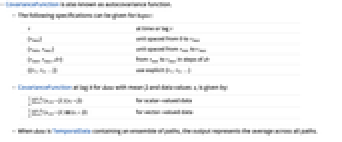
CovarianceFunctionは自己共分散関数としても知られている．
hspec に使用可能な指定

	τ	時間あるいは遅れ τ で
	{τ_max}	0から τ_maxまで等間隔で
	{τ_min,τ_max}	τ_minから τ_maxまで等間隔で
	{τ_min,τ_max,d τ}	τ_minから τ_maxまで刻み幅 d τ で
	{{τ₁,τ₂,…}}	明示的な{τ₁,τ₂,…}を使う

平均，データ値 x_iの data について，遅れ h におけるCovarianceFunctionは以下で与えられる．
(x_i+h- )(x_i-) スカラー値データについて

ベクトル値データについて
data が経路集合を含むTemporalDataの場合，出力はすべての経路の平均を表す．
時間 t における平均関数 μ[t]および値 x[t]の過程 proc のCovarianceFunctionは以下で与えられる．
Expectation[(x[s]-μ[s])(x[t]-μ[t])] スカラー値過程について

Expectation[(x[s]-μ[s])⊗(x[t]-μ[t])] ベクトル値過程について
記号 ⊗ はKroneckerProductを表す．
CovarianceFunction[proc,h]は proc が弱定常過程でCovarianceFunction[proc,h,0]と等しいときにのみ定義される．
過程 proc はARMAProcessやWienerProcessのような任意のランダム過程である．

例題

すべて開くすべて閉じる

例 (4)

遅れ2における共分散関数を推定する：

Wolfram Language code: CovarianceFunction[{2, 3, 4, 3}, 2]

自己回帰時系列からのランダムサンプルについてのサンプルの共分散関数：

Wolfram Language code: data = RandomFunction[ARProcess[{.2, .3, .4}, 1], {1, 10 ^ 4}];

Wolfram Language code: ListPlot[CovarianceFunction[data, {20}], Filling -> Axis, PlotRange -> All]

離散時間過程の共分散関数を計算する：

Wolfram Language code: CovarianceFunction[BinomialProcess[p], s, t]

Wolfram Language code: DiscretePlot3D[Evaluate[% /. {p -> 2 / 3}], {s, 0, 10}, {t, 0, 10}, ExtentSize -> 1 / 2, ColorFunction -> "Rainbow"]

連続時間過程の共分散関数を計算する：

Wolfram Language code: CovarianceFunction[WienerProcess[μ, σ], s, t]

Wolfram Language code: Plot3D[Evaluate[% /. {μ -> 1, σ -> 2}], {s, 0, 10}, {t, 0, 10}, ColorFunction -> "Rainbow"]

スコープ (13)

経験的推定値 (7)

遅れ9におけるデータの共分散関数を推定する：

Wolfram Language code: CovarianceFunction[Range[10], 9]

遅れ9までの共分散関数の経験的推定値を得る：

Wolfram Language code: CovarianceFunction[Range[10], {9}]

刻み幅2で遅れ1から9までの共分散関数を計算する：

Wolfram Language code: CovarianceFunction[Range[10], {1, 9, 2}]

時系列についての共分散関数を計算する：

Wolfram Language code:

ts = TemporalData[TimeSeries, {{{-2.9904395734335427, -1.5547517217370468, -2.007044987914736, 
    -0.7114933373063236, -1.5920036118254968, 0.23183536513859127, 0.056774681349179124, 
    0.32394041932443046, 0.10382798659711348, -0.684046765274114, - ... 1687325555, 
    3.410933732368106, 2.5200924558212163, 2.008558601261935, 0.43151331467691206, 
    0.6249727955196763}}, {{1, 1000, 1}}, 1, {"Continuous", 1}, {"Discrete", 1}, 1, 
  {ValueDimensions -> 1, ResamplingMethod -> None}}, False, 10.1];

複数の遅れについての時系列の共分散関数は，時系列として与えられる：

Wolfram Language code: cov = CovarianceFunction[ts, {100}]

Wolfram Language code: ListPlot[cov, Filling -> Axis]

経路の集合について共分散関数を推定する：

Wolfram Language code: data = RandomFunction[ARProcess[{.8}, 1], {0, 500}, 25]

Wolfram Language code: cov = CovarianceFunction[data, {50}];

Wolfram Language code: ListPlot[cov, Filling -> 0]

経験的な共分散関数と理論上の共分散関数を比べる：

Wolfram Language code: proc = MAProcess[{.4, .3, .5, .6, .3}, 1.];

Wolfram Language code: data = RandomFunction[proc, {0, 5000}];

Wolfram Language code:

ListPlot[CovarianceFunction[#, {10}]& /@ {proc, data}, Filling -> {1 -> {2}}, PlotStyle -> PointSize[Medium], PlotLegends -> {"process covariance", "sample covariance"}]

ベクトルデータについての相互共分散をプロットする：

Wolfram Language code:

proc = ARProcess[{{{.3, .1}, {.6, .3}}}, {{1, .3}, {.3, .6}}];
data = RandomFunction[proc, {100}];
cov = CovarianceFunction[data, {-6, 6}];

Wolfram Language code: Table[ListPlot[cov["Values"][[All, i, j]], Filling -> 0, PlotLabel -> {i, j}], {i, 1, 2}, {j, 1, 2}]

ランダム過程 (6)

弱定常離散時間過程の共分散関数：

Wolfram Language code: CovarianceFunction[ARProcess[{a}, σ^2], s, t]

Wolfram Language code:

DiscretePlot3D[Evaluate[% /. {a -> 2 / 3, σ -> 1}], {s, 0, 10}, {t, 0, 10}, ExtentSize -> 1 / 2, ColorFunction -> "Rainbow"]

共分散関数は反対角にのみ依存する：

Wolfram Language code: CovarianceFunction[ARProcess[{a}, σ^2], h]

Wolfram Language code:

DiscretePlot[Evaluate[% /. {a -> 2 / 3, σ -> 1}], {h, 0, 10}, ExtentSize -> 1 / 2, ColorFunction -> "Rainbow", AxesLabel -> {h, None}]

弱定常連続時間過程の共分散関数：

Wolfram Language code: CovarianceFunction[OrnsteinUhlenbeckProcess[μ, σ, θ], s, t]

Wolfram Language code: Plot3D[Evaluate[% /. {μ -> 1, σ -> 2, θ -> 1 / 3}], {s, 0, 10}, {t, 0, 10}, ColorFunction -> "Rainbow"]

共分散関数は反対角にのみ依存する：

Wolfram Language code: CovarianceFunction[OrnsteinUhlenbeckProcess[μ, σ, θ], h]

Wolfram Language code:

Plot[Evaluate[% /. {μ -> 1, σ -> 2, θ -> 1 / 3}], {h, 0, 10}, ColorFunction -> "Rainbow", Filling -> Axis, AxesLabel -> {h, None}]

弱定常ではない離散時間過程の共分散関数：

Wolfram Language code: CovarianceFunction[BinomialProcess[p], s, t]

Wolfram Language code:

DiscretePlot3D[Evaluate[% /. p -> 1 / 3], {s, 0, 10}, {t, 0, 10}, 
	ExtentSize -> 1 / 2, ColorFunction -> "Rainbow"]

共分散関数は，両方の時間引数に依存する：

Wolfram Language code: antidiagonals = CovarianceFunction[BinomialProcess[1 / 3], t, t + h]

Wolfram Language code:

DiscretePlot[Evaluate@Table[antidiagonals, {t, 1, 4}], {h, 0, 6}, ExtentSize -> 1 / 2, PlotLegends -> (Row[{"t = ", #}]& /@ Range[1, 4]), AxesLabel -> {h, None}]

弱定常ではない連続時間過程の共分散関数：

Wolfram Language code: CovarianceFunction[PoissonProcess[μ], s, t]

Wolfram Language code: Plot3D[Evaluate[% /. μ -> 3], {s, 0, 10}, {t, 0, 10}, ColorFunction -> "Rainbow"]

共分散関数は，両方の時間引数に依存する：

Wolfram Language code: antidiagonals = CovarianceFunction[PoissonProcess[3], t, t + h]

Wolfram Language code:

Plot[Evaluate@Table[antidiagonals, {t, 1, 4}], {h, 0, 6}, AxesLabel -> {h, None}, PlotLegends -> (Row[{"t = ", #}]& /@ Range[1, 4])]

いくつかの時系列過程の共分散関数：

Wolfram Language code:

proc1 = ARProcess[{.8}, 1];
proc2 = MAProcess[{-.4, -.7, .6, -1}, 1];
proc3 = SARMAProcess[{}, {}, {3, {.6}, {.1}}, 1];
proc4 = FARIMAProcess[{}, 1 / 3, {}, 1];

Wolfram Language code:

DiscretePlot[CovarianceFunction[#, h], {h, 0, 15}, ExtentSize -> 1 / 2, PlotRange -> All, PlotLabel -> Head[#]]& /@ {proc1, proc2, proc3, proc4}

ベクトルARProcessについての相互共分散プロット：

Wolfram Language code:

proc = ARProcess[{{{.3, .1}, {.6, .3}}}, {{1, .3}, {.3, .6}}];
cov = CovarianceFunction[proc, h];

Wolfram Language code: Table[DiscretePlot[cov[[i, j]], {h, -6, 6}, ExtentSize -> 1 / 2, PlotLabel -> {i, j}], {i, 1, 2}, {j, 1, 2}]

アプリケーション (1)

次のデータはMAProcessあるいはARProcessのどちらを使った場合に最もうまくモデル化ができるかを考える：

Wolfram Language code:

ListLinePlot[data = TemporalData[TimeSeries, {{{-1.4735257611469446, -0.9158187257309729, -1.9060205147226934, 
    -1.6174582169404574, -2.633459084244463, -2.104839842098871, -2.8701276893108894, 
    -2.4118183939601607, -0.5125633448622677, -1.2356329399850385, 1. ... 26394036266876, -0.16380797769527589, 0.3559909972777121, 
    1.5343047104249412, 0.10763337590714506}}, {{0, 100, 1}}, 1, {"Continuous", 1}, 
  {"Discrete", 1}, 1, {ResamplingMethod -> {"Interpolation", InterpolationOrder -> 1}}}, False, 
 10.1]]

もとになっている過程をサンプル経路から決定するのは難しい：

Wolfram Language code: candidates = {MAProcess[{.5, .4}, 1], ARProcess[{.5, .4}, 1]};

Wolfram Language code: SeedRandom[2];ListLinePlot[RandomFunction[#, {0, 100}]]& /@ candidates

データの共分散関数は徐々に減衰する：

Wolfram Language code: ListPlot[CovarianceFunction[data, {10}], Filling -> 0]

ARProcessは明らかにMAProcessよりもよいモデル候補である：

Wolfram Language code: ListPlot[CovarianceFunction[#, {10}], PlotLabel -> Head[#], Filling -> 0]& /@ candidates

特性と関係 (14)

サンプル共分散関数は，過程の共分散関数のバイアス推定器である：

Wolfram Language code:

proc = ARMAProcess[1, {5 / 6, -1 / 6}, {2 / 3}, 1];
paths = RandomFunction[proc, {0, n = 10}, 10 ^ 3];

サンプル共分散関数を計算する：

Wolfram Language code: CovarianceFunction[paths, {10}]

Wolfram Language code: scov = TimeSeriesMapThread[#2(n + 1) / (n + 1 - #1)&, %]

過程の共分散関数：

Wolfram Language code: cov = CovarianceFunction[proc, {10}]

両関数をプロットする：

Wolfram Language code: ListPlot[{scov, cov}, Filling -> 0, PlotLegends -> {"sample covariance", "process covariance"}]

過程の共分散関数はCovariance行列の非対角項である：

Wolfram Language code: 𝒫 = WienerProcess[μ, σ];

Wolfram Language code: Covariance[𝒫[{s, t}], 1, 2]

Wolfram Language code: CovarianceFunction[𝒫, s, t]

Wolfram Language code: Simplify[%% - %, 0 < s < t]

遅れ0におけるサンプルの共分散関数は，分散推定器である：

Wolfram Language code:

data = Range[10];
evar1 = CovarianceFunction[data, 0]

Varianceを使って推定値と比べる：

Wolfram Language code: evar2 = Variance[data]

スケーリングの因数は異なる：

Wolfram Language code: (10 evar1) / (9evar2)

サンプルの共分散関数は，CorrelationFunctionに関連している：

Wolfram Language code: data = Range[10];

Wolfram Language code: CovarianceFunction[data, {9}]

スケールされたサンプルの相関関数：

Wolfram Language code: CorrelationFunction[data, {9}] (CovarianceFunction[data, 0])

Wolfram Language code: % - %%

サンプルの共分散関数は，AbsoluteCorrelationFunctionに関連している：

Wolfram Language code:

data = Range[10];
n = Length[data];

Wolfram Language code: CovarianceFunction[data, {n - 1}]

Wolfram Language code: AbsoluteCorrelationFunction[data - Mean[data], {n - 1}]

Wolfram Language code: % - %%

Expectationを使って共分散関数を計算する：

Wolfram Language code:

𝒫 = WienerProcess[μ, σ];
m[s_] := Mean[𝒫[s]]

Wolfram Language code: Expectation[(x[s] - m[s])(x[t] - m[t]), x𝒫, Assumptions -> s > 0 && t > 0]

Wolfram Language code: CovarianceFunction[𝒫, s, t]

Wolfram Language code: Simplify[% - %%, 0 < s < t]

等しい時間に対する共分散関数は，Varianceに簡約される：

Wolfram Language code: 𝒫 = OrnsteinUhlenbeckProcess[μ, σ, θ];

Wolfram Language code: CovarianceFunction[𝒫, t, t]

Wolfram Language code: Variance[𝒫[t]]

Wolfram Language code: % - %%

共分散関数は，AbsoluteCorrelationFunction に関連している：

Wolfram Language code: 𝒫 = WienerProcess[μ, σ];

Wolfram Language code: AbsoluteCorrelationFunction[𝒫, s, t]

については，平均関数はである：

Wolfram Language code: CovarianceFunction[𝒫, s, t] + Mean[𝒫[s]] Mean[𝒫[t]]

Wolfram Language code: % - %%

共分散関数はCovarianceに関連している：

Wolfram Language code: 𝒫 = WienerProcess[μ, σ];

Wolfram Language code: CovarianceFunction[𝒫, s, t]

それは共分散行列中の非対角項である：

Wolfram Language code: Covariance[𝒫[{s, t}], 1, 2]

Wolfram Language code: Simplify[%% - %, 0 < s < t]

共分散関数は，CorrelationFunction に関連している：

Wolfram Language code:

𝒫 = PoissonProcess[μ];
sd[s_] := StandardDeviation[𝒫[s]]

Wolfram Language code: CorrelationFunction[𝒫, s, t]

については，標準偏差関数はである：

Wolfram Language code: CovarianceFunction[𝒫, s, t] / (sd[s] sd[t])

Wolfram Language code: % - %%//FullSimplify[#, s > 0 && t > 0]&

共分散関数は，ToInvertibleTimeSeriesについては不変である：

Wolfram Language code: TimeSeriesInvertibility[proc = MAProcess[{2, 4}, 1]]

Wolfram Language code: iproc = ToInvertibleTimeSeries@proc

Wolfram Language code: CovarianceFunction[#, s, t]& /@ {proc, iproc}

共分散関数は，中心に集めても不変である：

Wolfram Language code: data = RandomFunction[ARIMAProcess[{}, 1, {}, 1], {0, 100}];

データは非零の平均を持つ：

Wolfram Language code: Mean[data]

データを中心に集める：

Wolfram Language code: newdata = Standardize[data, Mean, 1&];

共分散関数を比べる：

Wolfram Language code: ListPlot[CovarianceFunction[#, {20}], Filling -> 0]& /@ {data, newdata}

時系列のPowerSpectralDensityは共分散関数を変換したものである：

Wolfram Language code:

proc = ARProcess[c, {a}, σ^2];
cf = CovarianceFunction[proc, h]

FourierSequenceTransformを使う：

Wolfram Language code: ft = FourierSequenceTransform[cf, h, z]

パワースペクトルと比較する：

Wolfram Language code: PowerSpectralDensity[proc, z]

Wolfram Language code: FullSimplify[% - ft]

データのPowerSpectralDensityはサンプル共分散関数を変換したものである：

Wolfram Language code:

sample = Range[20];
n = Length[sample];
cov = CovarianceFunction[sample, {n - 1}];
cov = Join[Reverse[Rest[cov]], cov];

ListFourierSequenceTransformを適用する：

Wolfram Language code: ListFourierSequenceTransform[cov, w, -n + 1]//ExpToTrig

SamplePowerSpectralDensityと比較する：

Wolfram Language code: PowerSpectralDensity[sample, w]

Wolfram Language code: % - %%//FullSimplify

考えられる問題 (1)

CovarianceFunctionの出力にはDifferenceRootが含まれることがある：

Wolfram Language code: CovarianceFunction[ARProcess[{a, b}, σ^2], t] //Simplify[#, t > 0]&

FunctionExpandを使って明示的なベキを回復する：

Wolfram Language code: %//FunctionExpand

Top

その他のラーニングリソース

テクニカルサポート

データサイエンス，金融，ビジネス

工学

科学とテクノロジー

教育のためのテクノロジー

教育イニシアチブ

使い始める

Grow Your Skills

Wolframと繋がる

大人用の教育プログラム

若者のための教育プログラム

読む

CovarianceFunction

詳細

例題

例 (4)

スコープ (13)

経験的推定値 (7)

ランダム過程 (6)

アプリケーション (1)

特性と関係 (14)

考えられる問題 (1)

テキスト

CMS

APA

BibTeX

BibLaTeX

	(x_i+h- )(x_i-)	スカラー値データについて
		ベクトル値データについて

	Expectation[(x[s]-μ[s])(x[t]-μ[t])]	スカラー値過程について
	Expectation[(x[s]-μ[s])⊗(x[t]-μ[t])]	ベクトル値過程について

CovarianceFunction

詳細

例題

例 (4)

スコープ (13)

経験的推定値 (7)

ランダム過程 (6)

アプリケーション (1)

特性と関係 (14)

考えられる問題 (1)

関連項目

関連するガイド

履歴

テキスト

CMS

APA

BibTeX

BibLaTeX