

CovarianceFunction[data,hspec]
估计数据 data 在滞后 hspec 处的协方差函数.
CovarianceFunction[proc,hspec]
表示随机过程 proc 在滞后 hspec 处的协方差函数.
CovarianceFunction[proc,s,t]
表示随机过程 proc 在时刻 s 和 t 的协方差函数.
CovarianceFunction
CovarianceFunction[data,hspec]
估计数据 data 在滞后 hspec 处的协方差函数.
CovarianceFunction[proc,hspec]
表示随机过程 proc 在滞后 hspec 处的协方差函数.
CovarianceFunction[proc,s,t]
表示随机过程 proc 在时刻 s 和 t 的协方差函数.
更多信息
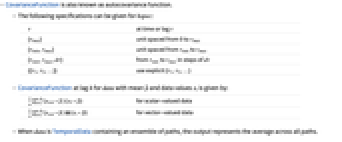
- CovarianceFunction 也被称为自协方差函数.
- 可以对 hspec 给出下列规范:
-
τ 在时刻或滞后 τ {τmax} 从 0 到 τmax 的间距单位 {τmin,τmax} 从 τmin 到 τmax 的间距单位 {τmin,τmax,d τ} 步长为 d τ,从 τmin 到 τmax {{τ1,τ2,…}} 使用显式 {τ1,τ2,…} - 对于 data,在滞后 h 的 CovarianceFunction 由下式给出,其中均值为
,数据值为 xi: -

(xi+h-
)(xi-
)对于标量值数据 
对于向量值数据 - 当 data 为包含一组路径的 TemporalData 时,输出表示所有路径的平均值.
- 过程 proc 的 CovarianceFunction,其中在时刻 t 的均值函数 μ[t] 和 x[t] 由以下各式给出:
-
Expectation[(x[s]-μ[s])(x[t]-μ[t])] 对于标量值过程 Expectation[(x[s]-μ[s])⊗(x[t]-μ[t])] 对于向量值过程 - 符号 ⊗ 表示 KroneckerProduct.
- CovarianceFunction[proc,h] 仅当 proc 是一个弱平稳过程的时候有定义,且等价于 CovarianceFunction[proc,h,0].
- 过程 proc 可以是诸如 ARMAProcess 和 WienerProcess 的任意随机过程.
范例
打开所有单元 关闭所有单元基本范例 (4)
CovarianceFunction[{2, 3, 4, 3}, 2]data = RandomFunction[ARProcess[{.2, .3, .4}, 1], {1, 10 ^ 4}];ListPlot[CovarianceFunction[data, {20}], Filling -> Axis, PlotRange -> All]CovarianceFunction[BinomialProcess[p], s, t]DiscretePlot3D[Evaluate[% /. {p -> 2 / 3}], {s, 0, 10}, {t, 0, 10}, ExtentSize -> 1 / 2, ColorFunction -> "Rainbow"]CovarianceFunction[WienerProcess[μ, σ], s, t]Plot3D[Evaluate[% /. {μ -> 1, σ -> 2}], {s, 0, 10}, {t, 0, 10}, ColorFunction -> "Rainbow"]范围 (13)
经验估计 (7)
CovarianceFunction[Range[10], 9]CovarianceFunction[Range[10], {9}]CovarianceFunction[Range[10], {1, 9, 2}]ts = TemporalData[TimeSeries, {{{-2.9904395734335427, -1.5547517217370468, -2.007044987914736,
-0.7114933373063236, -1.5920036118254968, 0.23183536513859127, 0.056774681349179124,
0.32394041932443046, 0.10382798659711348, -0.684046765274114, - ... 1687325555,
3.410933732368106, 2.5200924558212163, 2.008558601261935, 0.43151331467691206,
0.6249727955196763}}, {{1, 1000, 1}}, 1, {"Continuous", 1}, {"Discrete", 1}, 1,
{ValueDimensions -> 1, ResamplingMethod -> None}}, False, 10.1];cov = CovarianceFunction[ts, {100}]ListPlot[cov, Filling -> Axis]data = RandomFunction[ARProcess[{.8}, 1], {0, 500}, 25]cov = CovarianceFunction[data, {50}];ListPlot[cov, Filling -> 0]proc = MAProcess[{.4, .3, .5, .6, .3}, 1.];data = RandomFunction[proc, {0, 5000}];ListPlot[CovarianceFunction[#, {10}]& /@ {proc, data}, Filling -> {1 -> {2}}, PlotStyle -> PointSize[Medium], PlotLegends -> {"process covariance", "sample covariance"}]proc = ARProcess[{{{.3, .1}, {.6, .3}}}, {{1, .3}, {.3, .6}}];
data = RandomFunction[proc, {100}];
cov = CovarianceFunction[data, {-6, 6}];Table[ListPlot[cov["Values"][[All, i, j]], Filling -> 0, PlotLabel -> {i, j}], {i, 1, 2}, {j, 1, 2}]随机过程 (6)
CovarianceFunction[ARProcess[{a}, σ^2], s, t]DiscretePlot3D[Evaluate[% /. {a -> 2 / 3, σ -> 1}], {s, 0, 10}, {t, 0, 10}, ExtentSize -> 1 / 2, ColorFunction -> "Rainbow"]CovarianceFunction[ARProcess[{a}, σ^2], h]DiscretePlot[Evaluate[% /. {a -> 2 / 3, σ -> 1}], {h, 0, 10}, ExtentSize -> 1 / 2, ColorFunction -> "Rainbow", AxesLabel -> {h, None}]CovarianceFunction[OrnsteinUhlenbeckProcess[μ, σ, θ], s, t]Plot3D[Evaluate[% /. {μ -> 1, σ -> 2, θ -> 1 / 3}], {s, 0, 10}, {t, 0, 10}, ColorFunction -> "Rainbow"]CovarianceFunction[OrnsteinUhlenbeckProcess[μ, σ, θ], h]Plot[Evaluate[% /. {μ -> 1, σ -> 2, θ -> 1 / 3}], {h, 0, 10}, ColorFunction -> "Rainbow", Filling -> Axis, AxesLabel -> {h, None}]CovarianceFunction[BinomialProcess[p], s, t]DiscretePlot3D[Evaluate[% /. p -> 1 / 3], {s, 0, 10}, {t, 0, 10},
ExtentSize -> 1 / 2, ColorFunction -> "Rainbow"]antidiagonals = CovarianceFunction[BinomialProcess[1 / 3], t, t + h]DiscretePlot[Evaluate@Table[antidiagonals, {t, 1, 4}], {h, 0, 6}, ExtentSize -> 1 / 2, PlotLegends -> (Row[{"t = ", #}]& /@ Range[1, 4]), AxesLabel -> {h, None}]CovarianceFunction[PoissonProcess[μ], s, t]Plot3D[Evaluate[% /. μ -> 3], {s, 0, 10}, {t, 0, 10}, ColorFunction -> "Rainbow"]antidiagonals = CovarianceFunction[PoissonProcess[3], t, t + h]Plot[Evaluate@Table[antidiagonals, {t, 1, 4}], {h, 0, 6}, AxesLabel -> {h, None}, PlotLegends -> (Row[{"t = ", #}]& /@ Range[1, 4])]proc1 = ARProcess[{.8}, 1];
proc2 = MAProcess[{-.4, -.7, .6, -1}, 1];
proc3 = SARMAProcess[{}, {}, {3, {.6}, {.1}}, 1];
proc4 = FARIMAProcess[{}, 1 / 3, {}, 1];DiscretePlot[CovarianceFunction[#, h], {h, 0, 15}, ExtentSize -> 1 / 2, PlotRange -> All, PlotLabel -> Head[#]]& /@ {proc1, proc2, proc3, proc4}向量 ARProcess 的互协方差图:
proc = ARProcess[{{{.3, .1}, {.6, .3}}}, {{1, .3}, {.3, .6}}];
cov = CovarianceFunction[proc, h];Table[DiscretePlot[cov[[i, j]], {h, -6, 6}, ExtentSize -> 1 / 2, PlotLabel -> {i, j}], {i, 1, 2}, {j, 1, 2}]应用 (1)
确定下列数据是用 MAProcess 模拟还是用 ARProcess 模拟效果最好:
ListLinePlot[data = TemporalData[TimeSeries, {{{-1.4735257611469446, -0.9158187257309729, -1.9060205147226934,
-1.6174582169404574, -2.633459084244463, -2.104839842098871, -2.8701276893108894,
-2.4118183939601607, -0.5125633448622677, -1.2356329399850385, 1. ... 26394036266876, -0.16380797769527589, 0.3559909972777121,
1.5343047104249412, 0.10763337590714506}}, {{0, 100, 1}}, 1, {"Continuous", 1},
{"Discrete", 1}, 1, {ResamplingMethod -> {"Interpolation", InterpolationOrder -> 1}}}, False,
10.1]]candidates = {MAProcess[{.5, .4}, 1], ARProcess[{.5, .4}, 1]};SeedRandom[2];ListLinePlot[RandomFunction[#, {0, 100}]]& /@ candidatesListPlot[CovarianceFunction[data, {10}], Filling -> 0]显然,ARProcess 是一个比 MAProcess 更好的候选模型:
ListPlot[CovarianceFunction[#, {10}], PlotLabel -> Head[#], Filling -> 0]& /@ candidates属性和关系 (14)
proc = ARMAProcess[1, {5 / 6, -1 / 6}, {2 / 3}, 1];
paths = RandomFunction[proc, {0, n = 10}, 10 ^ 3];CovarianceFunction[paths, {10}]scov = TimeSeriesMapThread[#2(n + 1) / (n + 1 - #1)&, %]cov = CovarianceFunction[proc, {10}]ListPlot[{scov, cov}, Filling -> 0, PlotLegends -> {"sample covariance", "process covariance"}]过程的协方差函数是 Covariance 矩阵的非对角线项:
𝒫 = WienerProcess[μ, σ];Covariance[𝒫[{s, t}], 1, 2]CovarianceFunction[𝒫, s, t]Simplify[%% - %, 0 < s < t]data = Range[10];
evar1 = CovarianceFunction[data, 0]利用 Variance 与估计比较:
evar2 = Variance[data](10 evar1) / (9evar2)样本协方差函数与 CorrelationFunction 有关:
data = Range[10];CovarianceFunction[data, {9}]CorrelationFunction[data, {9}] (CovarianceFunction[data, 0])% - %%样本协方差函数与 AbsoluteCorrelationFunction 有关:
data = Range[10];
n = Length[data];CovarianceFunction[data, {n - 1}]AbsoluteCorrelationFunction[data - Mean[data], {n - 1}]% - %%使用 Expectation 计算协方差函数:
𝒫 = WienerProcess[μ, σ];
m[s_] := Mean[𝒫[s]]Expectation[(x[s] - m[s])(x[t] - m[t]), x𝒫, Assumptions -> s > 0 && t > 0]CovarianceFunction[𝒫, s, t]Simplify[% - %%, 0 < s < t]相同时间的协方差函数减少为 Variance:
𝒫 = OrnsteinUhlenbeckProcess[μ, σ, θ];CovarianceFunction[𝒫, t, t]Variance[𝒫[t]]% - %%协方差函数
与 AbsoluteCorrelationFunction
有关:
𝒫 = WienerProcess[μ, σ];AbsoluteCorrelationFunction[𝒫, s, t]CovarianceFunction[𝒫, s, t] + Mean[𝒫[s]] Mean[𝒫[t]]% - %%协方差函数与 Covariance 有关:
𝒫 = WienerProcess[μ, σ];CovarianceFunction[𝒫, s, t]Covariance[𝒫[{s, t}], 1, 2]Simplify[%% - %, 0 < s < t]协方差函数
与 CorrelationFunction
有关:
𝒫 = PoissonProcess[μ];
sd[s_] := StandardDeviation[𝒫[s]]CorrelationFunction[𝒫, s, t]CovarianceFunction[𝒫, s, t] / (sd[s] sd[t])% - %%//FullSimplify[#, s > 0 && t > 0]&协方差函数对于 ToInvertibleTimeSeries 是不变的:
TimeSeriesInvertibility[proc = MAProcess[{2, 4}, 1]]iproc = ToInvertibleTimeSeries@procCovarianceFunction[#, s, t]& /@ {proc, iproc}data = RandomFunction[ARIMAProcess[{}, 1, {}, 1], {0, 100}];Mean[data]newdata = Standardize[data, Mean, 1&];ListPlot[CovarianceFunction[#, {20}], Filling -> 0]& /@ {data, newdata}时间序列的 PowerSpectralDensity 是协方差函数的变换:
proc = ARProcess[c, {a}, σ^2];
cf = CovarianceFunction[proc, h]ft = FourierSequenceTransform[cf, h, z]PowerSpectralDensity[proc, z]FullSimplify[% - ft]数据的 PowerSpectralDensity 是样本协方差函数的变换:
sample = Range[20];
n = Length[sample];
cov = CovarianceFunction[sample, {n - 1}];
cov = Join[Reverse[Rest[cov]], cov];应用 ListFourierSequenceTransform:
ListFourierSequenceTransform[cov, w, -n + 1]//ExpToTrig与 SamplePowerSpectralDensity 比较:
PowerSpectralDensity[sample, w]% - %%//FullSimplify可能存在的问题 (1)
CovarianceFunction 输出可包含 DifferenceRoot:
CovarianceFunction[ARProcess[{a, b}, σ^2], t] //Simplify[#, t > 0]&使用 FunctionExpand 来恢复显式的幂:
%//FunctionExpand文本
Wolfram Research (2012),CovarianceFunction,Wolfram 语言函数,https://reference.wolfram.com/language/ref/CovarianceFunction.html.
CMS
Wolfram 语言. 2012. "CovarianceFunction." Wolfram 语言与系统参考资料中心. Wolfram Research. https://reference.wolfram.com/language/ref/CovarianceFunction.html.
APA
Wolfram 语言. (2012). CovarianceFunction. Wolfram 语言与系统参考资料中心. 追溯自 https://reference.wolfram.com/language/ref/CovarianceFunction.html 年
BibTeX
@misc{reference.wolfram_2026_covariancefunction, author="Wolfram Research", title="{CovarianceFunction}", year="2012", howpublished="\url{https://reference.wolfram.com/language/ref/CovarianceFunction.html}", note=[Accessed: 14-September-2026]}
BibLaTeX
@online{reference.wolfram_2026_covariancefunction, organization={Wolfram Research}, title={CovarianceFunction}, year={2012}, url={https://reference.wolfram.com/language/ref/CovarianceFunction.html}, note=[Accessed: 14-September-2026]}


