Wolfram 语言与系统参考资料中心

Power

参见
- Sqrt
- Exp
- CubeRoot
- Surd
- PowerExpand
- PowerMod
- Log
- Log10
- Log2
- LogLogPlot
- FactorialPower
- PowerRange
- PolygonalNumber
- GeneralizedPower
相关指南
技术笔记
- 算术
- 参见
  - Sqrt
  - Exp
  - CubeRoot
  - Surd
  - PowerExpand
  - PowerMod
  - Log
  - Log10
  - Log2
  - LogLogPlot
  - FactorialPower
  - PowerRange
  - PolygonalNumber
  - GeneralizedPower
- 相关指南
- 技术笔记
  - 算术

Power

x^y

给出关于的次幂.

背景

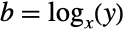
Power 是一个计算表达式给定幂次的数学函数，称为指数函数. 表达式 Power[x,y] 通常通过速记语法被表示为 x^y 的形式或输入为 2D 排版形式 x^y. 一个数的一次方等于它自身（），而 1 的任意复数次方都等于 1（）. 指数函数的反函数由 Log 给出，所以求满足方程的值，主解是 .
求一个表达式二次幂的操作被称为“平方”而求一个表达式三次幂的操作被称为“立方”. 结合包含幂次的量的运算法则被称为指数律，而把一个底数提升到给定幂次的过程被称为乘方. 许多涉及 Power、Exp、Log 和相关函数的表达式会被自动化简而其余则可能需要用 Simplify 或 FullSimplify 化简. PowerExpand 可被用于进行形式化的展开和相关化简，而 ExpToTrig 可被用于求 Power 表达式的三角函数形式.
函数 Sqrt[x] 是用 Power[x,1/2] 表示的. 使用自然对数 E 为底的乘幂可被输入为 Exp[x] 但实际是用 Power[E,x] 表示的.
对非整数的 y，Power[x,y] 在复 x 平面上对 y 由一个从到 0 的不连续的分支切割. 因为这个分支切割，对负实数值的 x 和正奇数 n，Power[x,1/n] 默认返回复数根而不是实数根. 要得到实数值的第 n 个根，可以用 Surd[x,n]. 特例 CubeRoot[x] 对应的是 Surd[x,3].

范例

打开所有单元关闭所有单元

基本范例 (6)

数值化计算：

Wolfram Language code: 2 ^ 100

用输入一个上标：

Wolfram Language code: 2^100

明确的 FullForm：

Wolfram Language code: Power[2, 100]

在实数的子集上绘图：

Wolfram Language code: Plot[Power[x, 3], {x, 0, 5}]

在复数的子集上绘图：

Wolfram Language code: ComplexPlot3D[z^3, {z, -3 - 3I, 3 + 3I}, PlotLegends -> Automatic]

在奇点处的渐近展开式：

Wolfram Language code: Series[Power[x^2 / 3], {x, -1, 3}, Assumptions -> Im[x] > 0]

范围 (46)

数值计算 (9)

数值化计算：

Wolfram Language code: Power[2., -1 / 2]

高精度计算：

Wolfram Language code: N[((12/17))^5, 50]

高效计算结果的前一百万位：

Wolfram Language code: res = N[Power[123, 4567890], 10 ^ 6];//Timing

必要时产生复数：

Wolfram Language code: (-5)^1 / 2

总是使用主根：

Wolfram Language code: (-1)^1 / 3

Wolfram Language code: N[%]

下面的式子遵循 Power 的广义定义，：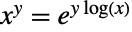

Wolfram Language code: %% == Exp[(1/3) Log[-1]]

可用 Surd 来获取实根：

Wolfram Language code: Surd[-1, 3]

复数输入：

Wolfram Language code: N[Power[2, I]]

Wolfram Language code: Power[I, 2]

Wolfram Language code: Power[2, I, 2]

Power 逐项作用于列表和矩阵的各个元素：

Wolfram Language code: {0, 1.5, I π, ∞}^1 / 2

Wolfram Language code: 2 ^ {1, 2, 3}

Wolfram Language code:

(⁠|   |    |
| :- | :- |
| 1 | u  |
| v | I  |⁠)^2//MatrixForm

Power 可与 Interval 和 CenteredInterval 对象一起使用：

Wolfram Language code: Interval[{1 / 3, 2}] ^ 3

Wolfram Language code: Pi ^ Interval[{2, 3.}]

Wolfram Language code: CenteredInterval[2, 1 / 100] ^ CenteredInterval[3, 1 / 100]

Wolfram Language code: CenteredInterval[2 + 3I, (1 + I) / 100] ^ CenteredInterval[3, (1 + I) / 100]

用 Around 计算普通的统计区间：

Wolfram Language code: Power[ 2, Around[2 / 3, 0.001]]

逐项计算数组中每个元素的值：

Wolfram Language code: Power[2, {{1 / 2, -1}, {-5 / 3, 1 / 2}}]

或用 MatrixFunction 计算矩阵形式的 Power 函数：

Wolfram Language code: MatrixFunction[Power[2, #]&, {{1 / 2, -1}, {-5 / 3, 1 / 2}}]//FullSimplify

特殊值 (4)

零处的值：

Wolfram Language code: Power[x, 0]

Wolfram Language code: Power[0, n]

取决于的实部，结果可以是 0 或无穷：

Wolfram Language code: {0^2, 0^-2}//Quiet

因此下式的结果不确定：

Wolfram Language code: Power[0, 0]//Quiet

无穷处的极限值：

Wolfram Language code: Limit[x ^ n, n -> ∞, Assumptions -> Abs[x] < 1]

Wolfram Language code: Limit[x ^ n, n -> ∞, Assumptions -> Abs[x] > 1]

符号计算：

Wolfram Language code: Power[2, y]

Wolfram Language code: Power[x, 5]

Wolfram Language code: Power[x, y, z]

求当 Power[x,3]=0.5，x 的值：

Wolfram Language code: xval = x /. FindRoot[Power[x, 3] == 0.5, {x, 0.1}]

可视化结果：

Wolfram Language code: Plot[Power[x, 3], {x, 0, 1}, Epilog -> Style[Point[{xval, Power[xval, 3]}], PointSize[Large], Red]]

可视化 (5)

n 取不同的整数值，在实数上绘制函数：

Wolfram Language code: Plot[{x^1, x^2, x^3, x^4}, {x, -1, 1}, PlotLegends -> "Expressions"]

绘制实域的实部和虚部：

Wolfram Language code: ReImPlot[x^2 / 3, {x, -4, 4}, PlotLegends -> Automatic]

在实数上比较 (Power[x,]) 和 (CubeRoot[x]) 的实部和虚部：

Wolfram Language code: ReImPlot[{x^(1/(3)), Surd[x, 3]}, {x, -4, 4}, PlotLegends -> Automatic]

绘制的实部：

Wolfram Language code: ComplexContourPlot[Re[(z)^5 / 2], {z, -3 - 3 I, 3 + 3I}, Contours -> 20]

绘制的虚部：

Wolfram Language code: ComplexContourPlot[Im[(z)^5 / 2], {z, -3 - 3 I, 3 + 3I}, Contours -> 20]

的极坐标图：

Wolfram Language code: PolarPlot[ϕ^3, {ϕ, 0, 8π}, Frame -> True]

函数的属性 (11)

当，为所有实定义：

Wolfram Language code: FunctionDomain[2^n, n]

只定义当时的整数：

Wolfram Language code: FunctionDomain[(-2)^n, n]

对于非零复数，它是的整个函数：

Wolfram Language code: FunctionDomain[(-2)^n, n, Complexes]

的函数范围：

Wolfram Language code: FunctionRange[2^n, n, y]

Wolfram Language code: FunctionRange[2^n, n, z, Complexes]

Power 是右结合：

Wolfram Language code: Power[x, y, z] === Power[x, Power[y, z]]

右侧的形式是首选形式：

Wolfram Language code: Power[x, y, z]//FullForm

Power 在复平面上第二个参数上是周期性的：

Wolfram Language code: FunctionPeriod[x ^ n, n, Complexes]

求分支切割处的极限：

Wolfram Language code: Limit[(-2 + ε) ^ (1 / 3), ε -> 0, Direction -> I]

Wolfram Language code: Limit[(-2 + ε) ^ (1 / 3), ε -> 0, Direction -> -I]

Wolfram Language code: N[{%, %%}]

对于固定的正整数，是的解析函数：

Wolfram Language code: FunctionAnalytic[x^n, x, Assumptions -> n∈ℤ && n > 0]

它不是解析函数，但对于负整数仍然是亚纯函数：

Wolfram Language code: FunctionMeromorphic[x^n, x, Assumptions -> n∈ℤ && n < 0]

对于非整数，它甚至不是亚纯函数：

Wolfram Language code: {FunctionMeromorphic[x^1 / 2, x], FunctionMeromorphic[x^-π, x]}

对于固定的非零实数，是的解析函数：

Wolfram Language code: FunctionAnalytic[b^x, x, Assumptions -> b∈ℝ && b ≠ 0]

作为二元函数，既不是解析函数也不是亚纯函数：

Wolfram Language code: {FunctionAnalytic[x^y, {x, y}], FunctionMeromorphic[x^y, {x, y}]}

对于，是增函数：

Wolfram Language code: FunctionMonotonicity[b^x, x, Assumptions -> b > 1, StrictInequalities -> True]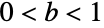

对于，它是减函数：

Wolfram Language code: FunctionMonotonicity[b^x, x, Assumptions -> 0 < b < 1, StrictInequalities -> True]

是单射的，除外:

Wolfram Language code: FunctionInjective[b^x, x, Assumptions -> b < -1 || b > 1 || -1 < b < 0 || 1 > b > 0]

可视化：

Wolfram Language code: Plot[{((1/4))^``x``, 5}, {x, -5, 5}]

对于的任何值，都不是实数上的满射函数：

Wolfram Language code: FunctionSurjective[b^x, x, Assumptions -> b > 1]

可视化：

Wolfram Language code: Plot[{4^``x``, -2}, {x, -5, 5}]

对于，为正：

Wolfram Language code: FunctionSign[b^``x``, x, Assumptions -> b > 0, StrictInequalities -> True]

对于偶数，是非负的：

Wolfram Language code: FunctionSign[x^n, x, Assumptions -> (n/2)∈ℤ && n > 0]

对于或，具有一般奇点：

Wolfram Language code: FunctionSingularities[x^n, x]

但是，当时，它在处是连续的：

Wolfram Language code: FunctionContinuous[{x ^ n, x ≥ 0}, x]//FullSimplify

对于，是凸函数：

Wolfram Language code: FunctionConvexity[b^x, x, Assumptions -> b > 0]

对于正偶数，是凸函数：

Wolfram Language code: FunctionConvexity[x^n, x, Assumptions -> (n/2)∈ℤ && n > 0]

微分 (4)

关于 x 的一阶导数：

Wolfram Language code: D[Power[x, n], x]

关于 x 的高阶导数：

Wolfram Language code: Table[D[Power[x, n], {x, k}], {k, 1, 4}]//FullSimplify

绘制关于 x 的高阶导数：

Wolfram Language code:

Plot[Evaluate[% /. n -> 4], {x, -3, 3}, PlotLegends -> {"First Derivative", "Second Derivative", "Third Derivative", "Fourth Derivative"}]

关于 x 的阶导数的公式：

Wolfram Language code: D[Power[x, n], {x, k}]// FullSimplify

关于第二个参数的导数：

Wolfram Language code: D[x^n, n]

阶导数：

Wolfram Language code: D[x^n, {n, k}]

积分 (3)

用 Integrate 计算不定积分：

Wolfram Language code: Integrate[x^y, x]// FullSimplify

验证反导数：

Wolfram Language code: FullSimplify[D[%, x]]// FullSimplify

定积分：

Wolfram Language code: Integrate[x^y, {x, 0, 10}, Assumptions -> Re[y] > -1]

更多积分：

Wolfram Language code: Integrate[x^y y^x, x]// FullSimplify

Wolfram Language code: Integrate[Log10[x] Power[E, x], {x, 0, E}]// FullSimplify

级数展开 (4)

用 Series 求泰勒展开式：

Wolfram Language code: Series[Power[y, x], {x, 0, 5}]

绘制附近的前三个近似式：

Wolfram Language code:

terms = Normal@Table[Series[Power[2, x], {x, 0, m}], {m, 1, 5, 2}];
Plot[{Power[2, x], terms}, {x, -10, 10}]

用 SeriesCoefficient 获取级数展开式的通项：

Wolfram Language code: SeriesCoefficient[Power[y, x], {x, 1, n}]

一阶傅立叶级数：

Wolfram Language code: FourierSeries[Power[y, x], x, 1]// FullSimplify

普通点处的泰勒展开式：

Wolfram Language code: Series[Power[y, x], {x, x0, 2}]// FullSimplify

函数恒等式和化简 (6)

主定义：

Wolfram Language code: Power[z, 0] == 1

Wolfram Language code: Power[z, k] == z Power[z, k - 1]

欧拉公式：

Wolfram Language code: ExpToTrig[Power[E, I x]]

与 Exp 函数的关系：

Wolfram Language code: Power[-1, a] == Exp[I a π]//FullSimplify

并不总是自动将嵌套的幂组合起来：

Wolfram Language code: (x ^ 2)^1 / 3

用 PowerExpand 强制进行组合：

Wolfram Language code: PowerExpand[%]

这可能会导致错误的结果：

Wolfram Language code: (x ^ 2)^1 / 3 == PowerExpand[x^2 / 3] /. x -> -1

也可以用含有合适假设的 Simplify：

Wolfram Language code: Simplify[(x ^ 2)^1 / 3, x∈Reals]

自动组合乘积：

Wolfram Language code: Power[x, a]Power[x, b]

假设 x 和 y 为实变量的情况下进行展开：

Wolfram Language code: ComplexExpand[Power[x + I y, k]]

应用 (5)

5% 的复利：

Wolfram Language code: Table[(1 + 0.05) ^ n, {n, 5}]

求与边为的正方体具有同样体积的球体的半径：

Wolfram Language code: Reduce[(4/3)Pi r ^ 3 == a ^ 3, r, Reals]

Wolfram Language code: ToRadicals[%, Assumptions -> a > 0]

Wolfram Language code: % /. a -> 1.

复逆幂的等高线图：

Wolfram Language code: ContourPlot[Re[2 ^ (1 / (0.1 + x + I y))], {x, -0.1, 0.1}, {y, -0.1, 0.1}]

求有理函数的用 Log 表示的的积分：

Wolfram Language code: Integrate[1 / (x ^ 2 - 1), x]

求解具有可变有理系数的微分方程：

Wolfram Language code: DSolve[{(1 + x^2) y''[x] + 2 x y'[x] == 0, y[0] == 0, y'[0] == 1}, y[x], x]

属性和关系 (27)

方根的等价形式：

Wolfram Language code: {x ^ (1 / 2), Sqrt[x], Sqrt[x]}

自动化简根的幂形式：

Wolfram Language code: (z ^ (1 / 3)) ^ 3

不能自动化简根的幂形式：

Wolfram Language code: (z ^ 3) ^ (1 / 3)

Wolfram Language code: (z ^ 3) ^ (1 / 3) /. z -> -1

使用 Power[x,1/n] 或求主值负根：

Wolfram Language code: (-16.)^1 / 4

Wolfram Language code: -32.^(1/(5))

使用 Surd[x,n] 求 n 次方实根：

Wolfram Language code: Surd[-16., 4]

Wolfram Language code: Surd[-32., 5]

有假设条件的化简：

Wolfram Language code: Simplify[(z ^ 3) ^ (1 / 3), z > 0]

用 PowerExpand 处理正式化简：

Wolfram Language code: PowerExpand[(z ^ 3) ^ (1 / 3)]

获得对所有复数有效的结果：

Wolfram Language code: PowerExpand[(z ^ 3) ^ (1 / 3), Assumptions -> {}]

Wolfram Language code: PiecewiseExpand[%, Assumptions -> -Pi < Arg[z] ≤ Pi]

用 ExpToTrig 获得三角形式：

Wolfram Language code: (-1) ^ (1 / 7)

Wolfram Language code: ExpToTrig[(-1) ^ (1 / 7)]

化简成单个根：

Wolfram Language code: RootReduce[2 ^ (1 / 2) + 5 ^ (1 / 5)]

用 Solve 或 Root 求所有根：

Wolfram Language code: sol = Solve[x ^ 6 == 1, x]

Wolfram Language code: root = Table[Root[# ^ 6 - 1&, m], {m, 6}]

虽然表达形式和顺序不同，但这些是相同的根：

Wolfram Language code: Sort[ExpToTrig[x /. sol]] == Sort[root]

用 Expand 将多项式的幂展开：

Wolfram Language code: (1 + x) ^ 10

Wolfram Language code: Expand[(1 + x) ^ 10]

将幂自动应用到级数：

Wolfram Language code: Series[Exp[x], {x, 0, 5}]

Wolfram Language code: % ^ 4

关于幂的方程有无穷多的解：

Wolfram Language code: Solve[a ^ x == b, x]

Wolfram Language code: Reduce[a ^ x == b, x]//TraditionalForm

倒数、平方根等自动转换为幂：

Wolfram Language code: 1 / x ^ 2//FullForm

Wolfram Language code: Sqrt[x]//FullForm

将指数转换为幂：

Wolfram Language code: Exp[x] // FullForm

与的幂的匹配：

Wolfram Language code: Cases[{1 / x, 1, Sqrt[x], x, x ^ 2, x ^ 3}, x ^ _]

包含：

Wolfram Language code: Cases[{1 / x, 1, Sqrt[x], x, x ^ 2, x ^ 3}, x ^ _.]

在复平面上对于分数幂的分支线结果：

Wolfram Language code: Plot3D[Im[(x + I y) ^ (1 / 3)], {x, -3, 3}, {y, -2, 2}]

测试幂是否是代数：

Wolfram Language code: (2 + Sqrt[3]) ^ (1 / 3)∈Algebraics

Wolfram Language code: (Pi) ^ (1 / 3)∈Algebraics

积分：

Wolfram Language code: ∫x^aa^xⅆx

积分转换：

Wolfram Language code: LaplaceTransform[t^n, t, s]

Wolfram Language code: FourierTransform[1 / t ^ 2, t, s]

求和：

Wolfram Language code: Underoverscript[∑, k = Subscript[k, 1], Subscript[k, 2]]k^a

微分方程：

Wolfram Language code: DSolve[z Derivative[1][w][z] - a w[z] == 0, w[z], z]

在许多数学函数的特例中显示 Power：

Wolfram Language code: {HypergeometricPFQ[{-a}, {}, 1 - z], Hypergeometric2F1[-a, b, b, 1 - z], MeijerG[{{1 + a}, {}}, {{0}, {}}, z - 1]}

Power 可被表示为 DifferenceRoot：

Wolfram Language code: DifferenceRootReduce[Power[k, 2], k]

Wolfram Language code: DifferenceRootReduce[Power[z, k], k]

Power 的级数展开式中的一般项：

Wolfram Language code: SeriesCoefficient[Power[a, x], {x, 0, n}]

Power 的母函数：

Wolfram Language code: GeneratingFunction[Power[n, k], n, x]

Wolfram Language code: Series[%, {x, 0, 10}]

FindSequenceFunction 可以识别 Power 序列：

Wolfram Language code: Table[Power[n, 5], {n, 10}]

Wolfram Language code: FindSequenceFunction[%, n]

Power 的指数母函数：

Wolfram Language code: ExponentialGeneratingFunction[Power[k, n], n, x]

用 GeneralizedPower 表示任意二进制运算的整数幂：

Wolfram Language code: GeneralizedPower[NonCommutativeMultiply, x + y, 3]

Power 是 Times 的 GeneralizedPower：

Wolfram Language code: GeneralizedPower[Times, x, k]

可能存在的问题 (13)

Power 通常计算主根：

Wolfram Language code: (-1) ^ (1 / 3)

Wolfram Language code: N[%]

一般幂不是根的逆：

Wolfram Language code: (z ^ 3) ^ (1 / 3)

Wolfram Language code: (z ^ 3) ^ (1 / 3) /. z -> -1

Wolfram Language code: PowerExpand[(z ^ 3) ^ (1 / 3)]

对于近似数，生成虚部：

Wolfram Language code: ((-1.) ^ (1 / 3)) ^ 3

Wolfram Language code: ((N[-1, 20]) ^ (1 / 3)) ^ 3

用 Chop 删除较小的虚部：

Wolfram Language code: Chop[%]

分支线使得这个函数不连续：

Wolfram Language code: Plot[Sqrt[z ^ 2] / z, {z, -1, 1}]

它的导数一般为 0：

Wolfram Language code: D[Sqrt[z ^ 2] / z, z]

机器精度在分支线上给出错误的数值结果：

Wolfram Language code: N[(-2 + I ((Pi + 1) ^ 2 - Pi ^ 2 - 2Pi - 1 - Exp[-Pi ^ 4])) ^ (1 / 3)]

Wolfram Language code: N[(-2 + I ((Pi + 1) ^ 2 - Pi ^ 2 - 2Pi - 1 - Exp[-Pi ^ 4])) ^ (1 / 3), 8]

机器数输入可以给出任意精度的结果：

Wolfram Language code: 5 ^ 5 ^ 5.

Wolfram Language code: MachineNumberQ[%]

幂可以非常大：

Wolfram Language code: 2 ^ 2 ^ 20.

某些幂对于计算过大：

Wolfram Language code: 2 ^ 2 ^ 100.

幂可以给出不确定的表达式：

Wolfram Language code: 0 ^ 0

每个结果的精度由零的精度确定：

Wolfram Language code: {x ^ 0, x ^ 0.0, x ^ 0``10}

1 的符号幂仅当 1 为精确值或机器精度数的情况下计算：

Wolfram Language code: {1 ^ x, 1.0 ^ x, 1``10 ^ x}

数值幂某些时候不能求解：

Wolfram Language code: (Pi ^ 2 + 2Pi + 1 - (Pi + 1) ^ 2 + Exp[-1000]) ^ 0

机器精度的数值计算是不充分的：

Wolfram Language code: N[%]

更高的内部精度求出结果：

Wolfram Language code: Block[{$MaxExtraPrecision = 10 ^ 4}, N[%%, 20]]

非有理幂不能在级数中使用：

Wolfram Language code: Series[x ^ Sqrt[2] Sin[x], {x, 0, 5}]

Wolfram Language code: Head[%]

Power 按元素作用于矩阵：

Wolfram Language code: {{1, 2}, {3, 4}} ^ 2

对于矩阵幂用 MatrixPower：

Wolfram Language code: MatrixPower[{{1, 2}, {3, 4}}, 2]

巧妙范例 (3)

绘制连续幂：

Wolfram Language code: Plot[Evaluate[Table[x ^ n, {n, 10}]], {x, -1.2, 1.2}]

产生塔状的连续幂：

Wolfram Language code: NestList[z ^ #&, z, 6]

参数为塔状幂的等高线图：

Wolfram Language code:

ContourPlot[Evaluate[Sin[Arg[z^z^z^z /. z -> x + I y] / 2]], {x, -1, 1}, {y, -1, 1}, ColorFunction -> Hue, ContourStyle -> None, Exclusions -> {}]

的塔状的幂：

Wolfram Language code: ListPlot[Abs[NestList[I ^ #&, 1, 50]]]

求极限：

Wolfram Language code: FixedPoint[SetPrecision[I ^ #, 16]&, 1]

对极限求解：

Wolfram Language code: Solve[I ^ x == x, x]

Wolfram Language code: N[%, 16]

Top

更多学习资源

技术支持

数据科学、金融与商业

工程

科学与技术

教育科技

教育举措

开始

提高你的技能

与我们合作

成人教育计划

青少年教育计划

欢迎阅读

Power

更多信息

背景

范例

基本范例 (6)

范围 (46)

数值计算 (9)

特殊值 (4)

可视化 (5)

函数的属性 (11)

微分 (4)

积分 (3)

级数展开 (4)

函数恒等式和化简 (6)

应用 (5)

属性和关系 (27)

可能存在的问题 (13)

巧妙范例 (3)

文本

CMS

APA

BibTeX

BibLaTeX

Power

更多信息

背景

范例

基本范例 (6)

范围 (46)

数值计算 (9)

特殊值 (4)

可视化 (5)

函数的属性 (11)

微分 (4)

积分 (3)

级数展开 (4)

函数恒等式和化简 (6)

应用 (5)

属性和关系 (27)

可能存在的问题 (13)

巧妙范例 (3)

参见

技术笔记

相关指南

相关链接

历史

文本

CMS

APA

BibTeX

BibLaTeX